6. Learning to Classify Text
Detecting patterns is a central part of Natural Language Processing. Words ending in -ed tend to be past tense verbs (5.). Frequent use of will is indicative of news text (3). These observable patterns — word structure and word frequency — happen to correlate with particular aspects of meaning, such as tense and topic. But how did we know where to start looking, which aspects of form to associate with which aspects of meaning?
The goal of this chapter is to answer the following questions:
- How can we identify particular features of language data that are salient for classifying it?
- How can we construct models of language that can be used to perform language processing tasks automatically?
- What can we learn about language from these models?
Along the way we will study some important machine learning techniques, including decision trees, naive Bayes' classifiers, and maximum entropy classifiers. We will gloss over the mathematical and statistical underpinnings of these techniques, focusing instead on how and when to use them (see the Further Readings section for more technical background). Before looking at these methods, we first need to appreciate the broad scope of this topic.
1 Supervised Classification
Classification is the task of choosing the correct class label for a given input. In basic classification tasks, each input is considered in isolation from all other inputs, and the set of labels is defined in advance. Some examples of classification tasks are:
- Deciding whether an email is spam or not.
- Deciding what the topic of a news article is, from a fixed list of topic areas such as "sports," "technology," and "politics."
- Deciding whether a given occurrence of the word bank is used to refer to a river bank, a financial institution, the act of tilting to the side, or the act of depositing something in a financial institution.
The basic classification task has a number of interesting variants. For example, in multi-class classification, each instance may be assigned multiple labels; in open-class classification, the set of labels is not defined in advance; and in sequence classification, a list of inputs are jointly classified.
A classifier is called supervised if it is built based on training corpora containing the correct label for each input. The framework used by supervised classification is shown in 1.1.
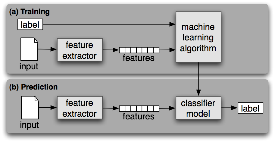
Figure 1.1: Supervised Classification. (a) During training, a feature extractor is used to convert each input value to a feature set. These feature sets, which capture the basic information about each input that should be used to classify it, are discussed in the next section. Pairs of feature sets and labels are fed into the machine learning algorithm to generate a model. (b) During prediction, the same feature extractor is used to convert unseen inputs to feature sets. These feature sets are then fed into the model, which generates predicted labels.
In the rest of this section, we will look at how classifiers can be employed to solve a wide variety of tasks. Our discussion is not intended to be comprehensive, but to give a representative sample of tasks that can be performed with the help of text classifiers.
1.1 Gender Identification
In 4 we saw that male and female names have some distinctive characteristics. Names ending in a, e and i are likely to be female, while names ending in k, o, r, s and t are likely to be male. Let's build a classifier to model these differences more precisely.
The first step in creating a classifier is deciding what features of the input are relevant, and how to encode those features. For this example, we'll start by just looking at the final letter of a given name. The following feature extractor function builds a dictionary containing relevant information about a given name:
|
The returned dictionary, known as a feature set, maps from feature names to their values. Feature names are case-sensitive strings that typically provide a short human-readable description of the feature, as in the example 'last_letter'. Feature values are values with simple types, such as booleans, numbers, and strings.
Note
Most classification methods require that features be encoded using simple value types, such as booleans, numbers, and strings. But note that just because a feature has a simple type, this does not necessarily mean that the feature's value is simple to express or compute. Indeed, it is even possible to use very complex and informative values, such as the output of a second supervised classifier, as features.
Now that we've defined a feature extractor, we need to prepare a list of examples and corresponding class labels.
|
Next, we use the feature extractor to process the names data, and divide the resulting list of feature sets into a training set and a test set. The training set is used to train a new "naive Bayes" classifier.
|
We will learn more about the naive Bayes classifier later in the chapter. For now, let's just test it out on some names that did not appear in its training data:
|
Observe that these character names from The Matrix are correctly classified. Although this science fiction movie is set in 2199, it still conforms with our expectations about names and genders. We can systematically evaluate the classifier on a much larger quantity of unseen data:
|
Finally, we can examine the classifier to determine which features it found most effective for distinguishing the names' genders:
|
This listing shows that the names in the training set that end in "a" are female 33 times more often than they are male, but names that end in "k" are male 32 times more often than they are female. These ratios are known as likelihood ratios, and can be useful for comparing different feature-outcome relationships.
Note
Your Turn: Modify the gender_features() function to provide the classifier with features encoding the length of the name, its first letter, and any other features that seem like they might be informative. Retrain the classifier with these new features, and test its accuracy.
When working with large corpora, constructing a single list that contains the features of every instance can use up a large amount of memory. In these cases, use the function nltk.classify.apply_features, which returns an object that acts like a list but does not store all the feature sets in memory:
|
1.2 Choosing The Right Features
Selecting relevant features and deciding how to encode them for a learning method can have an enormous impact on the learning method's ability to extract a good model. Much of the interesting work in building a classifier is deciding what features might be relevant, and how we can represent them. Although it's often possible to get decent performance by using a fairly simple and obvious set of features, there are usually significant gains to be had by using carefully constructed features based on a thorough understanding of the task at hand.
Typically, feature extractors are built through a process of trial-and-error, guided by intuitions about what information is relevant to the problem. It's common to start with a "kitchen sink" approach, including all the features that you can think of, and then checking to see which features actually are helpful. We take this approach for name gender features in 1.2.
| ||
| ||
Example 1.2 (code_gender_features_overfitting.py): Figure 1.2: A Feature Extractor that Overfits Gender Features. The feature sets returned by this feature extractor contain a large number of specific features, leading to overfitting for the relatively small Names Corpus. |
However, there are usually limits to the number of features that you should use with a given learning algorithm — if you provide too many features, then the algorithm will have a higher chance of relying on idiosyncrasies of your training data that don't generalize well to new examples. This problem is known as overfitting, and can be especially problematic when working with small training sets. For example, if we train a naive Bayes classifier using the feature extractor shown in 1.2, it will overfit the relatively small training set, resulting in a system whose accuracy is about 1% lower than the accuracy of a classifier that only pays attention to the final letter of each name:
|
Once an initial set of features has been chosen, a very productive method for refining the feature set is error analysis. First, we select a development set, containing the corpus data for creating the model. This development set is then subdivided into the training set and the dev-test set.
|
The training set is used to train the model, and the dev-test set is used to perform error analysis. The test set serves in our final evaluation of the system. For reasons discussed below, it is important that we employ a separate dev-test set for error analysis, rather than just using the test set. The division of the corpus data into different subsets is shown in 1.3.
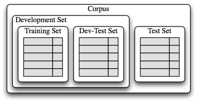
Figure 1.3: Organization of corpus data for training supervised classifiers. The corpus data is divided into two sets: the development set, and the test set. The development set is often further subdivided into a training set and a dev-test set.
Having divided the corpus into appropriate datasets, we train a model
using the training set ![[1]](callouts/callout1.gif) , and then run it on the
dev-test set
, and then run it on the
dev-test set ![[2]](callouts/callout2.gif) .
.
Using the dev-test set, we can generate a list of the errors that the classifier makes when predicting name genders:
|
We can then examine individual error cases where the model predicted the wrong label, and try to determine what additional pieces of information would allow it to make the right decision (or which existing pieces of information are tricking it into making the wrong decision). The feature set can then be adjusted accordingly. The names classifier that we have built generates about 100 errors on the dev-test corpus:
|
Looking through this list of errors makes it clear that some suffixes that are more than one letter can be indicative of name genders. For example, names ending in yn appear to be predominantly female, despite the fact that names ending in n tend to be male; and names ending in ch are usually male, even though names that end in h tend to be female. We therefore adjust our feature extractor to include features for two-letter suffixes:
|
Rebuilding the classifier with the new feature extractor, we see that the performance on the dev-test dataset improves by almost 2 percentage points (from 76.5% to 78.2%):
|
This error analysis procedure can then be repeated, checking for patterns in the errors that are made by the newly improved classifier. Each time the error analysis procedure is repeated, we should select a different dev-test/training split, to ensure that the classifier does not start to reflect idiosyncrasies in the dev-test set.
But once we've used the dev-test set to help us develop the model, we can no longer trust that it will give us an accurate idea of how well the model would perform on new data. It is therefore important to keep the test set separate, and unused, until our model development is complete. At that point, we can use the test set to evaluate how well our model will perform on new input values.
1.3 Document Classification
In 1, we saw several examples of corpora where documents have been labeled with categories. Using these corpora, we can build classifiers that will automatically tag new documents with appropriate category labels. First, we construct a list of documents, labeled with the appropriate categories. For this example, we've chosen the Movie Reviews Corpus, which categorizes each review as positive or negative.
|
Next, we define a feature extractor for documents, so the classifier
will know which aspects of the data it should pay attention to
(1.4). For document topic identification, we can
define a feature for each word, indicating whether the document
contains that word. To limit the number of features that the
classifier needs to process, we begin by constructing a list of the
2000 most frequent words in the overall corpus
. We can then define a feature extractor
that simply checks whether each of these
words is present in a given document.
| ||
| ||
Example 1.4 (code_document_classify_fd.py): Figure 1.4: A feature extractor for document classification, whose features indicate whether or not individual words are present in a given document. |
Note
The reason that we compute the set of all words in a document in
![[3]](callouts/callout3.gif) , rather than just checking if
word in document, is
that checking whether a word occurs in a set is much faster than
checking whether it occurs in a list (4.7).
, rather than just checking if
word in document, is
that checking whether a word occurs in a set is much faster than
checking whether it occurs in a list (4.7).
Now that we've defined our feature extractor, we can use it to train a
classifier to label new movie reviews (1.5). To
check how reliable the resulting classifier is, we compute its
accuracy on the test set . And once again,
we can use show_most_informative_features() to find out which
features the classifier found to be most informative
.
| ||
| ||
Example 1.5 (code_document_classify_use.py): Figure 1.5: Training and testing a classifier for document classification. |
Apparently in this corpus, a review that mentions "Seagal" is almost 8 times more likely to be negative than positive, while a review that mentions "Damon" is about 6 times more likely to be positive.
1.4 Part-of-Speech Tagging
In 5. we built a regular expression tagger that chooses a part-of-speech tag for a word by looking at the internal make-up of the word. However, this regular expression tagger had to be hand-crafted. Instead, we can train a classifier to work out which suffixes are most informative. Let's begin by finding out what the most common suffixes are:
|
|
Next, we'll define a feature extractor function which checks a given word for these suffixes:
|
Feature extraction functions behave like tinted glasses, highlighting some of the properties (colors) in our data and making it impossible to see other properties. The classifier will rely exclusively on these highlighted properties when determining how to label inputs. In this case, the classifier will make its decisions based only on information about which of the common suffixes (if any) a given word has.
Now that we've defined our feature extractor, we can use it to train a new "decision tree" classifier (to be discussed in 4):
|
|
|
|
One nice feature of decision tree models is that they are often fairly easy to interpret — we can even instruct NLTK to print them out as pseudocode:
|
Here, we can see that the classifier begins by checking whether a word ends with a comma — if so, then it will receive the special tag ",". Next, the classifier checks if the word ends in "the", in which case it's almost certainly a determiner. This "suffix" gets used early by the decision tree because the word "the" is so common. Continuing on, the classifier checks if the word ends in "s". If so, then it's most likely to receive the verb tag VBZ (unless it's the word "is", which has a special tag BEZ), and if not, then it's most likely a noun (unless it's the punctuation mark "."). The actual classifier contains further nested if-then statements below the ones shown here, but the depth=4 argument just displays the top portion of the decision tree.
1.5 Exploiting Context
By augmenting the feature extraction function, we could modify this part-of-speech tagger to leverage a variety of other word-internal features, such as the length of the word, the number of syllables it contains, or its prefix. However, as long as the feature extractor just looks at the target word, we have no way to add features that depend on the context that the word appears in. But contextual features often provide powerful clues about the correct tag — for example, when tagging the word "fly," knowing that the previous word is "a" will allow us to determine that it is functioning as a noun, not a verb.
In order to accommodate features that depend on a word's context, we must revise the pattern that we used to define our feature extractor. Instead of just passing in the word to be tagged, we will pass in a complete (untagged) sentence, along with the index of the target word. This approach is demonstrated in 1.6, which employs a context-dependent feature extractor to define a part of speech tag classifier.
| ||
| ||
Example 1.6 (code_suffix_pos_tag.py): Figure 1.6: A part-of-speech classifier whose feature detector examines the context in which a word appears in order to determine which part of speech tag should be assigned. In particular, the identity of the previous word is included as a feature. |
It is clear that exploiting contextual features improves the performance of our part-of-speech tagger. For example, the classifier learns that a word is likely to be a noun if it comes immediately after the word "large" or the word "gubernatorial". However, it is unable to learn the generalization that a word is probably a noun if it follows an adjective, because it doesn't have access to the previous word's part-of-speech tag. In general, simple classifiers always treat each input as independent from all other inputs. In many contexts, this makes perfect sense. For example, decisions about whether names tend to be male or female can be made on a case-by-case basis. However, there are often cases, such as part-of-speech tagging, where we are interested in solving classification problems that are closely related to one another.
1.6 Sequence Classification
In order to capture the dependencies between related classification tasks, we can use joint classifier models, which choose an appropriate labeling for a collection of related inputs. In the case of part-of-speech tagging, a variety of different sequence classifier models can be used to jointly choose part-of-speech tags for all the words in a given sentence.
One sequence classification strategy, known as consecutive classification or greedy sequence classification, is to find the most likely class label for the first input, then to use that answer to help find the best label for the next input. The process can then be repeated until all of the inputs have been labeled. This is the approach that was taken by the bigram tagger from 5, which began by choosing a part-of-speech tag for the first word in the sentence, and then chose the tag for each subsequent word based on the word itself and the predicted tag for the previous word.
This strategy is demonstrated in 1.7.
First, we must
augment our feature extractor function to take a history
argument, which provides a list of the tags that we've predicted for
the sentence so far .
Each tag in history corresponds with a word in sentence. But
note that history will only contain tags for words we've already
classified, that is, words to the left of the target word. Thus, while it is
possible to look at some features of words to the right
of the target word, it is not possible to look at the tags for those
words (since we haven't generated them yet).
Having defined a feature extractor, we can proceed to build our
sequence classifier . During training, we use
the annotated tags to
provide the appropriate history to the feature extractor, but when
tagging new sentences, we generate the history list based on the
output of the tagger itself.
| ||
| ||
Example 1.7 (code_consecutive_pos_tagger.py): Figure 1.7: Part of Speech Tagging with a Consecutive Classifier |
1.7 Other Methods for Sequence Classification
One shortcoming of this approach is that we commit to every decision that we make. For example, if we decide to label a word as a noun, but later find evidence that it should have been a verb, there's no way to go back and fix our mistake. One solution to this problem is to adopt a transformational strategy instead. Transformational joint classifiers work by creating an initial assignment of labels for the inputs, and then iteratively refining that assignment in an attempt to repair inconsistencies between related inputs. The Brill tagger, described in (1), is a good example of this strategy.
Another solution is to assign scores to all of the possible sequences of part-of-speech tags, and to choose the sequence whose overall score is highest. This is the approach taken by Hidden Markov Models. Hidden Markov Models are similar to consecutive classifiers in that they look at both the inputs and the history of predicted tags. However, rather than simply finding the single best tag for a given word, they generate a probability distribution over tags. These probabilities are then combined to calculate probability scores for tag sequences, and the tag sequence with the highest probability is chosen. Unfortunately, the number of possible tag sequences is quite large. Given a tag set with 30 tags, there are about 600 trillion (3010) ways to label a 10-word sentence. In order to avoid considering all these possible sequences separately, Hidden Markov Models require that the feature extractor only look at the most recent tag (or the most recent n tags, where n is fairly small). Given that restriction, it is possible to use dynamic programming (4.7) to efficiently find the most likely tag sequence. In particular, for each consecutive word index i, a score is computed for each possible current and previous tag. This same basic approach is taken by two more advanced models, called Maximum Entropy Markov Models and Linear-Chain Conditional Random Field Models; but different algorithms are used to find scores for tag sequences.
2 Further Examples of Supervised Classification
2.1 Sentence Segmentation
Sentence segmentation can be viewed as a classification task for punctuation: whenever we encounter a symbol that could possibly end a sentence, such as a period or a question mark, we have to decide whether it terminates the preceding sentence.
The first step is to obtain some data that has already been segmented into sentences and convert it into a form that is suitable for extracting features:
|
Here, tokens is a merged list of tokens from the individual sentences, and boundaries is a set containing the indexes of all sentence-boundary tokens. Next, we need to specify the features of the data that will be used in order to decide whether punctuation indicates a sentence-boundary:
|
Based on this feature extractor, we can create a list of labeled featuresets by selecting all the punctuation tokens, and tagging whether they are boundary tokens or not:
|
Using these featuresets, we can train and evaluate a punctuation classifier:
|
To use this classifier to perform sentence segmentation, we simply check each punctuation mark to see whether it's labeled as a boundary; and divide the list of words at the boundary marks. The listing in 2.1 shows how this can be done.
| ||
Example 2.1 (code_classification_based_segmenter.py): Figure 2.1: Classification Based Sentence Segmenter |
2.2 Identifying Dialogue Act Types
When processing dialogue, it can be useful to think of utterances as a type of action performed by the speaker. This interpretation is most straightforward for performative statements such as "I forgive you" or "I bet you can't climb that hill." But greetings, questions, answers, assertions, and clarifications can all be thought of as types of speech-based actions. Recognizing the dialogue acts underlying the utterances in a dialogue can be an important first step in understanding the conversation.
The NPS Chat Corpus, which was demonstrated in 1, consists of over 10,000 posts from instant messaging sessions. These posts have all been labeled with one of 15 dialogue act types, such as "Statement," "Emotion," "ynQuestion", and "Continuer." We can therefore use this data to build a classifier that can identify the dialogue act types for new instant messaging posts. The first step is to extract the basic messaging data. We will call xml_posts() to get a data structure representing the XML annotation for each post:
|
Next, we'll define a simple feature extractor that checks what words the post contains:
|
Finally, we construct the training and testing data by applying the feature extractor to each post (using post.get('class') to get a post's dialogue act type), and create a new classifier:
|
2.3 Recognizing Textual Entailment
Recognizing textual entailment (RTE) is the task of determining whether a given piece of text T entails another text called the "hypothesis" (as already discussed in 5). To date, there have been four RTE Challenges, where shared development and test data is made available to competing teams. Here are a couple of examples of text/hypothesis pairs from the Challenge 3 development dataset. The label True indicates that the entailment holds, and False, that it fails to hold.
Challenge 3, Pair 34 (True)
T: Parviz Davudi was representing Iran at a meeting of the Shanghai Co-operation Organisation (SCO), the fledgling association that binds Russia, China and four former Soviet republics of central Asia together to fight terrorism.
H: China is a member of SCO.
Challenge 3, Pair 81 (False)
T: According to NC Articles of Organization, the members of LLC company are H. Nelson Beavers, III, H. Chester Beavers and Jennie Beavers Stewart.
H: Jennie Beavers Stewart is a share-holder of Carolina Analytical Laboratory.
It should be emphasized that the relationship between text and hypothesis is not intended to be logical entailment, but rather whether a human would conclude that the text provides reasonable evidence for taking the hypothesis to be true.
We can treat RTE as a classification task, in which we try to predict the True/False label for each pair. Although it seems likely that successful approaches to this task will involve a combination of parsing, semantics and real world knowledge, many early attempts at RTE achieved reasonably good results with shallow analysis, based on similarity between the text and hypothesis at the word level. In the ideal case, we would expect that if there is an entailment, then all the information expressed by the hypothesis should also be present in the text. Conversely, if there is information found in the hypothesis that is absent from the text, then there will be no entailment.
In our RTE feature detector (2.2), we let words (i.e., word types) serve as proxies for information, and our features count the degree of word overlap, and the degree to which there are words in the hypothesis but not in the text (captured by the method hyp_extra()). Not all words are equally important — Named Entity mentions such as the names of people, organizations and places are likely to be more significant, which motivates us to extract distinct information for words and nes (Named Entities). In addition, some high frequency function words are filtered out as "stopwords".
| [xx] | give some intro to RTEFeatureExtractor?? |
| ||
Example 2.2 (code_rte_features.py): Figure 2.2: "Recognizing Text Entailment" Feature Extractor. The RTEFeatureExtractor class builds a bag of words for both the text and the hypothesis after throwing away some stopwords, then calculates overlap and difference. |
To illustrate the content of these features, we examine some attributes of the text/hypothesis Pair 34 shown earlier:
|
These features indicate that all important words in the hypothesis are contained in the text, and thus there is some evidence for labeling this as True.
The module nltk.classify.rte_classify reaches just over 58% accuracy on the combined RTE test data using methods like these. Although this figure is not very impressive, it requires significant effort, and more linguistic processing, to achieve much better results.
2.4 Scaling Up to Large Datasets
Python provides an excellent environment for performing basic text processing and feature extraction. However, it is not able to perform the numerically intensive calculations required by machine learning methods nearly as quickly as lower-level languages such as C. Thus, if you attempt to use the pure-Python machine learning implementations (such as nltk.NaiveBayesClassifier) on large datasets, you may find that the learning algorithm takes an unreasonable amount of time and memory to complete.
If you plan to train classifiers with large amounts of training data or a large number of features, we recommend that you explore NLTK's facilities for interfacing with external machine learning packages. Once these packages have been installed, NLTK can transparently invoke them (via system calls) to train classifier models significantly faster than the pure-Python classifier implementations. See the NLTK webpage for a list of recommended machine learning packages that are supported by NLTK.
3 Evaluation
In order to decide whether a classification model is accurately capturing a pattern, we must evaluate that model. The result of this evaluation is important for deciding how trustworthy the model is, and for what purposes we can use it. Evaluation can also be an effective tool for guiding us in making future improvements to the model.
3.1 The Test Set
Most evaluation techniques calculate a score for a model by comparing the labels that it generates for the inputs in a test set (or evaluation set) with the correct labels for those inputs. This test set typically has the same format as the training set. However, it is very important that the test set be distinct from the training corpus: if we simply re-used the training set as the test set, then a model that simply memorized its input, without learning how to generalize to new examples, would receive misleadingly high scores.
When building the test set, there is often a trade-off between the amount of data available for testing and the amount available for training. For classification tasks that have a small number of well-balanced labels and a diverse test set, a meaningful evaluation can be performed with as few as 100 evaluation instances. But if a classification task has a large number of labels, or includes very infrequent labels, then the size of the test set should be chosen to ensure that the least frequent label occurs at least 50 times. Additionally, if the test set contains many closely related instances — such as instances drawn from a single document — then the size of the test set should be increased to ensure that this lack of diversity does not skew the evaluation results. When large amounts of annotated data are available, it is common to err on the side of safety by using 10% of the overall data for evaluation.
Another consideration when choosing the test set is the degree of similarity between instances in the test set and those in the development set. The more similar these two datasets are, the less confident we can be that evaluation results will generalize to other datasets. For example, consider the part-of-speech tagging task. At one extreme, we could create the training set and test set by randomly assigning sentences from a data source that reflects a single genre (news):
|
In this case, our test set will be very similar to our training set. The training set and test set are taken from the same genre, and so we cannot be confident that evaluation results would generalize to other genres. What's worse, because of the call to random.shuffle(), the test set contains sentences that are taken from the same documents that were used for training. If there is any consistent pattern within a document — say, if a given word appears with a particular part-of-speech tag especially frequently — then that difference will be reflected in both the development set and the test set. A somewhat better approach is to ensure that the training set and test set are taken from different documents:
|
If we want to perform a more stringent evaluation, we can draw the test set from documents that are less closely related to those in the training set:
|
If we build a classifier that performs well on this test set, then we can be confident that it has the power to generalize well beyond the data that it was trained on.
3.2 Accuracy
The simplest metric that can be used to evaluate a classifier, accuracy, measures the percentage of inputs in the test set that the classifier correctly labeled. For example, a name gender classifier that predicts the correct name 60 times in a test set containing 80 names would have an accuracy of 60/80 = 75%. The function nltk.classify.accuracy() will calculate the accuracy of a classifier model on a given test set:
|
When interpreting the accuracy score of a classifier, it is important to take into consideration the frequencies of the individual class labels in the test set. For example, consider a classifier that determines the correct word sense for each occurrence of the word bank. If we evaluate this classifier on financial newswire text, then we may find that the financial-institution sense appears 19 times out of 20. In that case, an accuracy of 95% would hardly be impressive, since we could achieve that accuracy with a model that always returns the financial-institution sense. However, if we instead evaluate the classifier on a more balanced corpus, where the most frequent word sense has a frequency of 40%, then a 95% accuracy score would be a much more positive result. (A similar issue arises when measuring inter-annotator agreement in 2.)
3.3 Precision and Recall
Another instance where accuracy scores can be misleading is in "search" tasks, such as information retrieval, where we are attempting to find documents that are relevant to a particular task. Since the number of irrelevant documents far outweighs the number of relevant documents, the accuracy score for a model that labels every document as irrelevant would be very close to 100%.
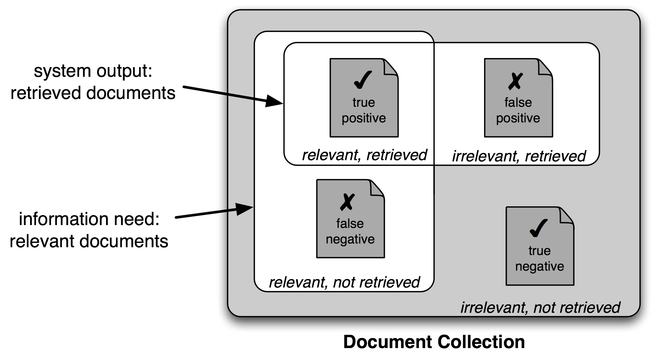
Figure 3.1: True and False Positives and Negatives
It is therefore conventional to employ a different set of measures for search tasks, based on the number of items in each of the four categories shown in 3.1:
- True positives are relevant items that we correctly identified as relevant.
- True negatives are irrelevant items that we correctly identified as irrelevant.
- False positives (or Type I errors) are irrelevant items that we incorrectly identified as relevant.
- False negatives (or Type II errors) are relevant items that we incorrectly identified as irrelevant.
Given these four numbers, we can define the following metrics:
- Precision, which indicates how many of the items that we identified were relevant, is TP/(TP+FP).
- Recall, which indicates how many of the relevant items that we identified, is TP/(TP+FN).
- The F-Measure (or F-Score), which combines the precision and recall to give a single score, is defined to be the harmonic mean of the precision and recall: (2 × Precision × Recall) / (Precision + Recall).
3.4 Confusion Matrices
When performing classification tasks with three or more labels, it can be informative to subdivide the errors made by the model based on which types of mistake it made. A confusion matrix is a table where each cell [i,j] indicates how often label j was predicted when the correct label was i. Thus, the diagonal entries (i.e., cells |ii|) indicate labels that were correctly predicted, and the off-diagonal entries indicate errors. In the following example, we generate a confusion matrix for the bigram tagger developed in 4:
|
The confusion matrix indicates that common errors include a substitution of NN for JJ (for 1.6% of words), and of NN for NNS (for 1.5% of words). Note that periods (.) indicate cells whose value is 0, and that the diagonal entries — which correspond to correct classifications — are marked with angle brackets. .. XXX explain use of "reference" in the legend above.
3.5 Cross-Validation
In order to evaluate our models, we must reserve a portion of the annotated data for the test set. As we already mentioned, if the test set is too small, then our evaluation may not be accurate. However, making the test set larger usually means making the training set smaller, which can have a significant impact on performance if a limited amount of annotated data is available.
One solution to this problem is to perform multiple evaluations on different test sets, then to combine the scores from those evaluations, a technique known as cross-validation. In particular, we subdivide the original corpus into N subsets called folds. For each of these folds, we train a model using all of the data except the data in that fold, and then test that model on the fold. Even though the individual folds might be too small to give accurate evaluation scores on their own, the combined evaluation score is based on a large amount of data, and is therefore quite reliable.
A second, and equally important, advantage of using cross-validation is that it allows us to examine how widely the performance varies across different training sets. If we get very similar scores for all N training sets, then we can be fairly confident that the score is accurate. On the other hand, if scores vary widely across the N training sets, then we should probably be skeptical about the accuracy of the evaluation score.
4 Decision Trees
In the next three sections, we'll take a closer look at three machine learning methods that can be used to automatically build classification models: decision trees, naive Bayes classifiers, and Maximum Entropy classifiers. As we've seen, it's possible to treat these learning methods as black boxes, simply training models and using them for prediction without understanding how they work. But there's a lot to be learned from taking a closer look at how these learning methods select models based on the data in a training set. An understanding of these methods can help guide our selection of appropriate features, and especially our decisions about how those features should be encoded. And an understanding of the generated models can allow us to extract information about which features are most informative, and how those features relate to one another.
A decision tree is a simple flowchart that selects labels for input values. This flowchart consists of decision nodes, which check feature values, and leaf nodes, which assign labels. To choose the label for an input value, we begin at the flowchart's initial decision node, known as its root node. This node contains a condition that checks one of the input value's features, and selects a branch based on that feature's value. Following the branch that describes our input value, we arrive at a new decision node, with a new condition on the input value's features. We continue following the branch selected by each node's condition, until we arrive at a leaf node which provides a label for the input value. 4.1 shows an example decision tree model for the name gender task.
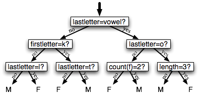
Figure 4.1: Decision Tree model for the name gender task. Note that tree diagrams are conventionally drawn "upside down," with the root at the top, and the leaves at the bottom.
Once we have a decision tree, it is straightforward to use it to assign labels to new input values. What's less straightforward is how we can build a decision tree that models a given training set. But before we look at the learning algorithm for building decision trees, we'll consider a simpler task: picking the best "decision stump" for a corpus. A decision stump is a decision tree with a single node that decides how to classify inputs based on a single feature. It contains one leaf for each possible feature value, specifying the class label that should be assigned to inputs whose features have that value. In order to build a decision stump, we must first decide which feature should be used. The simplest method is to just build a decision stump for each possible feature, and see which one achieves the highest accuracy on the training data, although there are other alternatives that we will discuss below. Once we've picked a feature, we can build the decision stump by assigning a label to each leaf based on the most frequent label for the selected examples in the training set (i.e., the examples where the selected feature has that value).
Given the algorithm for choosing decision stumps, the algorithm for growing larger decision trees is straightforward. We begin by selecting the overall best decision stump for the classification task. We then check the accuracy of each of the leaves on the training set. Leaves that do not achieve sufficient accuracy are then replaced by new decision stumps, trained on the subset of the training corpus that is selected by the path to the leaf. For example, we could grow the decision tree in 4.1 by replacing the leftmost leaf with a new decision stump, trained on the subset of the training set names that do not start with a "k" or end with a vowel or an "l."
4.1 Entropy and Information Gain
As was mentioned before, there are several methods for identifying the most informative feature for a decision stump. One popular alternative, called information gain, measures how much more organized the input values become when we divide them up using a given feature. To measure how disorganized the original set of input values are, we calculate entropy of their labels, which will be high if the input values have highly varied labels, and low if many input values all have the same label. In particular, entropy is defined as the sum of the probability of each label times the log probability of that same label:
| (1) | H = −Σl |in| labelsP(l) × log2P(l). |
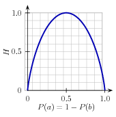
Figure 4.2: The entropy of labels in the name gender prediction task, as a function of the percentage of names in a given set that are male.
For example, 4.2 shows how the entropy of labels in the name gender prediction task depends on the ratio of male to female names. Note that if most input values have the same label (e.g., if P(male) is near 0 or near 1), then entropy is low. In particular, labels that have low frequency do not contribute much to the entropy (since P(l) is small), and labels with high frequency also do not contribute much to the entropy (since log2P(l) is small). On the other hand, if the input values have a wide variety of labels, then there are many labels with a "medium" frequency, where neither P(l) nor log2P(l) is small, so the entropy is high. 4.3 demonstrates how to calculate the entropy of a list of labels.
| ||
| ||
Example 4.3 (code_entropy.py): Figure 4.3: Calculating the Entropy of a List of Labels |
Once we have calculated the entropy of the original set of input values' labels, we can determine how much more organized the labels become once we apply the decision stump. To do so, we calculate the entropy for each of the decision stump's leaves, and take the average of those leaf entropy values (weighted by the number of samples in each leaf). The information gain is then equal to the original entropy minus this new, reduced entropy. The higher the information gain, the better job the decision stump does of dividing the input values into coherent groups, so we can build decision trees by selecting the decision stumps with the highest information gain.
Another consideration for decision trees is efficiency. The simple algorithm for selecting decision stumps described above must construct a candidate decision stump for every possible feature, and this process must be repeated for every node in the constructed decision tree. A number of algorithms have been developed to cut down on the training time by storing and reusing information about previously evaluated examples.
Decision trees have a number of useful qualities. To begin with, they're simple to understand, and easy to interpret. This is especially true near the top of the decision tree, where it is usually possible for the learning algorithm to find very useful features. Decision trees are especially well suited to cases where many hierarchical categorical distinctions can be made. For example, decision trees can be very effective at capturing phylogeny trees.
However, decision trees also have a few disadvantages. One problem is that, since each branch in the decision tree splits the training data, the amount of training data available to train nodes lower in the tree can become quite small. As a result, these lower decision nodes may
overfit the training set, learning patterns that reflect idiosyncrasies of the training set rather than linguistically significant patterns in the underlying problem. One solution to this problem is to stop dividing nodes once the amount of training data becomes too small. Another solution is to grow a full decision tree, but then to prune decision nodes that do not improve performance on a dev-test.
A second problem with decision trees is that they force features to be checked in a specific order, even when features may act relatively independently of one another. For example, when classifying documents into topics (such as sports, automotive, or murder mystery), features such as hasword(football) are highly indicative of a specific label, regardless of what other the feature values are. Since there is limited space near the top of the decision tree, most of these features will need to be repeated on many different branches in the tree. And since the number of branches increases exponentially as we go down the tree, the amount of repetition can be very large.
A related problem is that decision trees are not good at making use of features that are weak predictors of the correct label. Since these features make relatively small incremental improvements, they tend to occur very low in the decision tree. But by the time the decision tree learner has descended far enough to use these features, there is not enough training data left to reliably determine what effect they should have. If we could instead look at the effect of these features across the entire training set, then we might be able to make some conclusions about how they should affect the choice of label.
The fact that decision trees require that features be checked in a specific order limits their ability to exploit features that are relatively independent of one another. The naive Bayes classification method, which we'll discuss next, overcomes this limitation by allowing all features to act "in parallel."
5 Naive Bayes Classifiers
In naive Bayes classifiers, every feature gets a say in determining which label should be assigned to a given input value. To choose a label for an input value, the naive Bayes classifier begins by calculating the prior probability of each label, which is determined by checking frequency of each label in the training set. The contribution from each feature is then combined with this prior probability, to arrive at a likelihood estimate for each label. The label whose likelihood estimate is the highest is then assigned to the input value. 5.1 illustrates this process.
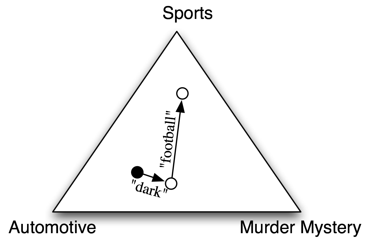
Figure 5.1: An abstract illustration of the procedure used by the naive Bayes classifier to choose the topic for a document. In the training corpus, most documents are automotive, so the classifier starts out at a point closer to the "automotive" label. But it then considers the effect of each feature. In this example, the input document contains the word "dark," which is a weak indicator for murder mysteries, but it also contains the word "football," which is a strong indicator for sports documents. After every feature has made its contribution, the classifier checks which label it is closest to, and assigns that label to the input.
Individual features make their contribution to the overall decision by "voting against" labels that don't occur with that feature very often. In particular, the likelihood score for each label is reduced by multiplying it by the probability that an input value with that label would have the feature. For example, if the word run occurs in 12% of the sports documents, 10% of the murder mystery documents, and 2% of the automotive documents, then the likelihood score for the sports label will be multiplied by 0.12; the likelihood score for the murder mystery label will be multiplied by 0.1, and the likelihood score for the automotive label will be multiplied by 0.02. The overall effect will be to reduce the score of the murder mystery label slightly more than the score of the sports label, and to significantly reduce the automotive label with respect to the other two labels. This process is illustrated in 5.2 and 5.3.
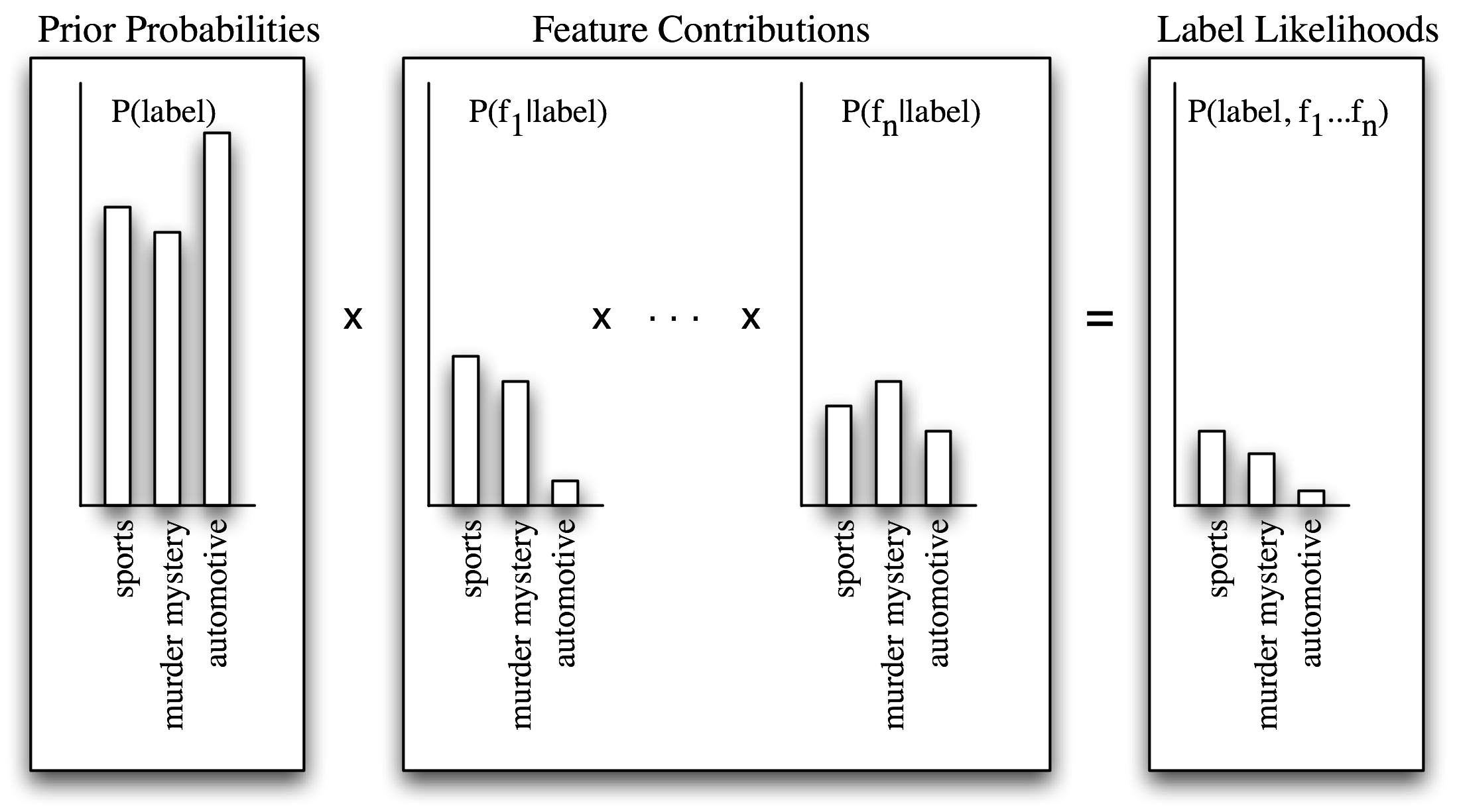
Figure 5.2: Calculating label likelihoods with naive Bayes. Naive Bayes begins by calculating the prior probability of each label, based on how frequently each label occurs in the training data. Every feature then contributes to the likelihood estimate for each label, by multiplying it by the probability that input values with that label will have that feature. The resulting likelihood score can be thought of as an estimate of the probability that a randomly selected value from the training set would have both the given label and the set of features, assuming that the feature probabilities are all independent.
5.1 Underlying Probabilistic Model
Another way of understanding the naive Bayes classifier is that it chooses the most likely label for an input, under the assumption that every input value is generated by first choosing a class label for that input value, and then generating each feature, entirely independent of every other feature. Of course, this assumption is unrealistic; features are often highly dependent on one another. We'll return to some of the consequences of this assumption at the end of this section. This simplifying assumption, known as the naive Bayes assumption (or independence assumption) makes it much easier to combine the contributions of the different features, since we don't need to worry about how they should interact with one another.
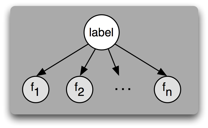
Figure 5.3: A Bayesian Network Graph illustrating the generative process that is assumed by the naive Bayes classifier. To generate a labeled input, the model first chooses a label for the input, then it generates each of the input's features based on that label. Every feature is assumed to be entirely independent of every other feature, given the label.
Based on this assumption, we can calculate an expression for P(label|features), the probability that an input will have a particular label given that it has a particular set of features. To choose a label for a new input, we can then simply pick the label l that maximizes P(l|features).
To begin, we note that P(label|features) is equal to the probability that an input has a particular label and the specified set of features, divided by the probability that it has the specified set of features:
| (2) | P(label|features) = P(features, label)/P(features) |
Next, we note that P(features) will be the same for every choice of label, so if we are simply interested in finding the most likely label, it suffices to calculate P(features, label), which we'll call the label likelihood.
Note
If we want to generate a probability estimate for each label, rather than just choosing the most likely label, then the easiest way to compute P(features) is to simply calculate the sum over labels of P(features, label):
| (3) | P(features) = Σl in| labels P(features, label) |
The label likelihood can be expanded out as the probability of the label times the probability of the features given the label:
| (4) | P(features, label) = P(label) × P(features|label) |
Furthermore, since the features are all independent of one another (given the label), we can separate out the probability of each individual feature:
| (5) | P(features, label) = P(label) × Prodf in| featuresP(f|label)` |
This is exactly the equation we discussed above for calculating the label likelihood: P(label) is the prior probability for a given label, and each P(f|label) is the contribution of a single feature to the label likelihood.
5.2 Zero Counts and Smoothing
The simplest way to calculate P(f|label), the contribution of a feature f toward the label likelihood for a label label, is to take the percentage of training instances with the given label that also have the given feature:
| (6) | P(f|label) = count(f, label) / count(label) |
However, this simple approach can become problematic when a feature never occurs with a given label in the training set. In this case, our calculated value for P(f|label) will be zero, which will cause the label likelihood for the given label to be zero. Thus, the input will never be assigned this label, regardless of how well the other features fit the label.
The basic problem here is with our calculation of P(f|label), the probability that an input will have a feature, given a label. In particular, just because we haven't seen a feature/label combination occur in the training set, doesn't mean it's impossible for that combination to occur. For example, we may not have seen any murder mystery documents that contained the word "football," but we wouldn't want to conclude that it's completely impossible for such documents to exist.
Thus, although count(f,label)/count(label) is a good estimate for P(f|label) when count(f, label) is relatively high, this estimate becomes less reliable when count(f) becomes smaller. Therefore, when building naive Bayes models, we usually employ more sophisticated techniques, known as smoothing techniques, for calculating P(f|label), the probability of a feature given a label. For example, the Expected Likelihood Estimation for the probability of a feature given a label basically adds 0.5 to each count(f,label) value, and the Heldout Estimation uses a heldout corpus to calculate the relationship between feature frequencies and feature probabilities. The nltk.probability module provides support for a wide variety of smoothing techniques.
5.3 Non-Binary Features
We have assumed here that each feature is binary, i.e. that each input either has a feature or does not. Label-valued features (e.g., a color feature which could be red, green, blue, white, or orange) can be converted to binary features by replacing them with binary features such as "color-is-red". Numeric features can be converted to binary features by binning, which replaces them with features such as "4<x<6".
Another alternative is to use regression methods to model the probabilities of numeric features. For example, if we assume that the height feature has a bell curve distribution, then we could estimate P(height|label) by finding the mean and variance of the heights of the inputs with each label. In this case, P(f=v|label) would not be a fixed value, but would vary depending on the value of v.
5.4 The Naivete of Independence
The reason that naive Bayes classifiers are called "naive" is that it's unreasonable to assume that all features are independent of one another (given the label). In particular, almost all real-world problems contain features with varying degrees of dependence on one another. If we had to avoid any features that were dependent on one another, it would be very difficult to construct good feature sets that provide the required information to the machine learning algorithm.
So what happens when we ignore the independence assumption, and use the naive Bayes classifier with features that are not independent? One problem that arises is that the classifier can end up "double-counting" the effect of highly correlated features, pushing the classifier closer to a given label than is justified.
To see how this can occur, consider a name gender classifier that contains two identical features, f1 and f2. In other words, f2 is an exact copy of f1, and contains no new information. When the classifier is considering an input, it will include the contribution of both f1 and f2 when deciding which label to choose. Thus, the information content of these two features will be given more weight than it deserves.
Of course, we don't usually build naive Bayes classifiers that contain two identical features. However, we do build classifiers that contain features which are dependent on one another. For example, the features ends-with(a) and ends-with(vowel) are dependent on one another, because if an input value has the first feature, then it must also have the second feature. For features like these, the duplicated information may be given more weight than is justified by the training set.
5.5 The Cause of Double-Counting
The reason for the double-counting problem is that during training, feature contributions are computed separately; but when using the classifier to choose labels for new inputs, those feature contributions are combined. One solution, therefore, is to consider the possible interactions between feature contributions during training. We could then use those interactions to adjust the contributions that individual features make.
To make this more precise, we can rewrite the equation used to calculate the likelihood of a label, separating out the contribution made by each feature (or label):
| (7) | P(features, label) = w[label] × Prodf |in| features w[f, label] |
Here, w[label] is the "starting score" for a given label, and w[f, label] is the contribution made by a given feature towards a label's likelihood. We call these values w[label] and w[f, label] the parameters or weights for the model. Using the naive Bayes algorithm, we set each of these parameters independently:
| (8) | w[label] = P(label) |
| (9) | w[f, label] = P(f|label) |
However, in the next section, we'll look at a classifier that considers the possible interactions between these parameters when choosing their values.
6 Maximum Entropy Classifiers
The Maximum Entropy classifier uses a model that is very similar to the model employed by the naive Bayes classifier. But rather than using probabilities to set the model's parameters, it uses search techniques to find a set of parameters that will maximize the performance of the classifier. In particular, it looks for the set of parameters that maximizes the total likelihood of the training corpus, which is defined as:
| (10) | P(features) = Σx |in| corpus P(label(x)|features(x)) |
Where P(label|features), the probability that an input whose features are features will have class label label, is defined as:
| (11) | P(label|features) = P(label, features) / Σlabel P(label, features) |
Because of the potentially complex interactions between the effects of related features, there is no way to directly calculate the model parameters that maximize the likelihood of the training set. Therefore, Maximum Entropy classifiers choose the model parameters using iterative optimization techniques, which initialize the model's parameters to random values, and then repeatedly refine those parameters to bring them closer to the optimal solution. These iterative optimization techniques guarantee that each refinement of the parameters will bring them closer to the optimal values, but do not necessarily provide a means of determining when those optimal values have been reached. Because the parameters for Maximum Entropy classifiers are selected using iterative optimization techniques, they can take a long time to learn. This is especially true when the size of the training set, the number of features, and the number of labels are all large.
Note
Some iterative optimization techniques are much faster than others. When training Maximum Entropy models, avoid the use of Generalized Iterative Scaling (GIS) or Improved Iterative Scaling (IIS), which are both considerably slower than the Conjugate Gradient (CG) and the BFGS optimization methods.
6.1 The Maximum Entropy Model
The Maximum Entropy classifier model is a generalization of the model used by the naive Bayes classifier. Like the naive Bayes model, the Maximum Entropy classifier calculates the likelihood of each label for a given input value by multiplying together the parameters that are applicable for the input value and label. The naive Bayes classifier model defines a parameter for each label, specifying its prior probability, and a parameter for each (feature, label) pair, specifying the contribution of individual features towards a label's likelihood.
In contrast, the Maximum Entropy classifier model leaves it up to the user to decide what combinations of labels and features should receive their own parameters. In particular, it is possible to use a single parameter to associate a feature with more than one label; or to associate more than one feature with a given label. This will sometimes allow the model to "generalize" over some of the differences between related labels or features.
Each combination of labels and features that receives its own parameter is called a joint-feature. Note that joint-features are properties of labeled values, whereas (simple) features are properties of unlabeled values.
Note
In literature that describes and discusses Maximum Entropy models, the term "features" often refers to joint-features; the term "contexts" refers to what we have been calling (simple) features.
Typically, the joint-features that are used to construct Maximum Entropy models exactly mirror those that are used by the naive Bayes model. In particular, a joint-feature is defined for each label, corresponding to w[label], and for each combination of (simple) feature and label, corresponding to w[f,label]. Given the joint-features for a Maximum Entropy model, the score assigned to a label for a given input is simply the product of the parameters associated with the joint-features that apply to that input and label:
| (12) | P(input, label) = Prodjoint-features(input,label) w[joint-feature] |
6.2 Maximizing Entropy
The intuition that motivates Maximum Entropy classification is that we should build a model that captures the frequencies of individual joint-features, without making any unwarranted assumptions. An example will help to illustrate this principle.
Suppose we are assigned the task of picking the correct word sense for a given word, from a list of ten possible senses (labeled A-J). At first, we are not told anything more about the word or the senses. There are many probability distributions that we could choose for the ten senses, such as:
| A | B | C | D | E | F | G | H | I | J | |
|---|---|---|---|---|---|---|---|---|---|---|
| (i) | 10% | 10% | 10% | 10% | 10% | 10% | 10% | 10% | 10% | 10% |
| (ii) | 5% | 15% | 0% | 30% | 0% | 8% | 12% | 0% | 6% | 24% |
| (iii) | 0% | 100% | 0% | 0% | 0% | 0% | 0% | 0% | 0% | 0% |
Although any of these distributions might be correct, we are likely to choose distribution (i), because without any more information, there is no reason to believe that any word sense is more likely than any other. On the other hand, distributions (ii) and (iii) reflect assumptions that are not supported by what we know.
One way to capture this intuition that distribution (i) is more "fair" than the other two is to invoke the concept of entropy. In the discussion of decision trees, we described entropy as a measure of how "disorganized" a set of labels was. In particular, if a single label dominates then entropy is low, but if the labels are more evenly distributed then entropy is high. In our example, we chose distribution (i) because its label probabilities are evenly distributed — in other words, because its entropy is high. In general, the Maximum Entropy principle states that, among the distributions that are consistent with what we know, we should choose the distribution whose entropy is highest.
Next, suppose that we are told that sense A appears 55% of the time. Once again, there are many distributions that are consistent with this new piece of information, such as:
| A | B | C | D | E | F | G | H | I | J | |
|---|---|---|---|---|---|---|---|---|---|---|
| (iv) | 55% | 45% | 0% | 0% | 0% | 0% | 0% | 0% | 0% | 0% |
| (v) | 55% | 5% | 5% | 5% | 5% | 5% | 5% | 5% | 5% | 5% |
| (vi) | 55% | 3% | 1% | 2% | 9% | 5% | 0% | 25% | 0% | 0% |
But again, we will likely choose the distribution that makes the fewest unwarranted assumptions — in this case, distribution (v).
Finally, suppose that we are told that the word "up" appears in the nearby context 10% of the time, and that when it does appear in the context there's an 80% chance that sense A or C will be used. In this case, we will have a harder time coming up with an appropriate distribution by hand; however, we can verify that the following distribution looks appropriate:
| A | B | C | D | E | F | G | H | I | J | ||
|---|---|---|---|---|---|---|---|---|---|---|---|
| (vii) | +up | 5.1% | 0.25% | 2.9% | 0.25% | 0.25% | 0.25% | 0.25% | 0.25% | 0.25% | 0.25% |
| ` ` | -up | 49.9% | 4.46% | 4.46% | 4.46% | 4.46% | 4.46% | 4.46% | 4.46% | 4.46% | 4.46% |
In particular, the distribution is consistent with what we know: if we add up the probabilities in column A, we get 55%; if we add up the probabilities of row 1, we get 10%; and if we add up the boxes for senses A and C in the +up row, we get 8% (or 80% of the +up cases). Furthermore, the remaining probabilities appear to be "evenly distributed."
Throughout this example, we have restricted ourselves to distributions that are consistent with what we know; among these, we chose the distribution with the highest entropy. This is exactly what the Maximum Entropy classifier does as well. In particular, for each joint-feature, the Maximum Entropy model calculates the "empirical frequency" of that feature — i.e., the frequency with which it occurs in the training set. It then searches for the distribution which maximizes entropy, while still predicting the correct frequency for each joint-feature.
6.3 Generative vs Conditional Classifiers
An important difference between the naive Bayes classifier and the Maximum Entropy classifier concerns the type of questions they can be used to answer. The naive Bayes classifier is an example of a generative classifier, which builds a model that predicts P(input, label), the joint probability of a (input, label) pair. As a result, generative models can be used to answer the following questions:
- What is the most likely label for a given input?
- How likely is a given label for a given input?
- What is the most likely input value?
- How likely is a given input value?
- How likely is a given input value with a given label?
- What is the most likely label for an input that might have one of two values (but we don't know which)?
The Maximum Entropy classifier, on the other hand, is an example of a conditional classifier. Conditional classifiers build models that predict P(label|input) — the probability of a label given the input value. Thus, conditional models can still be used to answer questions 1 and 2. However, conditional models can not be used to answer the remaining questions 3-6.
In general, generative models are strictly more powerful than conditional models, since we can calculate the conditional probability P(label|input) from the joint probability P(input, label), but not vice versa. However, this additional power comes at a price. Because the model is more powerful, it has more "free parameters" which need to be learned. However, the size of the training set is fixed. Thus, when using a more powerful model, we end up with less data that can be used to train each parameter's value, making it harder to find the best parameter values. As a result, a generative model may not do as good a job at answering questions 1 and 2 as a conditional model, since the conditional model can focus its efforts on those two questions. However, if we do need answers to questions like 3-6, then we have no choice but to use a generative model.
The difference between a generative model and a conditional model is analogous to the difference between a topographical map and a picture of a skyline. Although the topographical map can be used to answer a wider variety of questions, it is significantly more difficult to generate an accurate topographical map than it is to generate an accurate skyline.
7 Modeling Linguistic Patterns
Classifiers can help us to understand the linguistic patterns that occur in natural language, by allowing us to create explicit models that capture those patterns. Typically, these models are using supervised classification techniques, but it is also possible to build analytically motivated models. Either way, these explicit models serve two important purposes: they help us to understand linguistic patterns, and they can be used to make predictions about new language data.
The extent to which explicit models can give us insights into linguistic patterns depends largely on what kind of model is used. Some models, such as decision trees, are relatively transparent, and give us direct information about which factors are important in making decisions and about which factors are related to one another. Other models, such as multi-level neural networks, are much more opaque. Although it can be possible to gain insight by studying them, it typically takes a lot more work.
But all explicit models can make predictions about new "unseen" language data that was not included in the corpus used to build the model. These predictions can be evaluated to assess the accuracy of the model. Once a model is deemed sufficiently accurate, it can then be used to automatically predict information about new language data. These predictive models can be combined into systems that perform many useful language processing tasks, such as document classification, automatic translation, and question answering.
7.1 What do models tell us?
It's important to understand what we can learn about language from an automatically constructed model. One important consideration when dealing with models of language is the distinction between descriptive models and explanatory models. Descriptive models capture patterns in the data but they don't provide any information about why the data contains those patterns. For example, as we saw in 3.1, the synonyms absolutely and definitely are not interchangeable: we say absolutely adore not definitely adore, and definitely prefer not absolutely prefer. In contrast, explanatory models attempt to capture properties and relationships that cause the linguistic patterns. For example, we might introduce the abstract concept of "polar verb", as one that has an extreme meaning, and categorize some verb like adore and detest as polar. Our explanatory model would contain the constraint that absolutely can only combine with polar verbs, and definitely can only combine with non-polar verbs. In summary, descriptive models provide information about correlations in the data, while explanatory models go further to postulate causal relationships.
Most models that are automatically constructed from a corpus are descriptive models; in other words, they can tell us what features are relevant to a given pattern or construction, but they can't necessarily tell us how those features and patterns relate to one another. If our goal is to understand the linguistic patterns, then we can use this information about which features are related as a starting point for further experiments designed to tease apart the relationships between features and patterns. On the other hand, if we're just interested in using the model to make predictions (e.g., as part of a language processing system), then we can use the model to make predictions about new data without worrying about the details of underlying causal relationships.
8 Summary
- Modeling the linguistic data found in corpora can help us to understand linguistic patterns, and can be used to make predictions about new language data.
- Supervised classifiers use labeled training corpora to build models that predict the label of an input based on specific features of that input.
- Supervised classifiers can perform a wide variety of NLP tasks, including document classification, part-of-speech tagging, sentence segmentation, dialogue act type identification, and determining entailment relations, and many other tasks.
- When training a supervised classifier, you should split your corpus into three datasets: a training set for building the classifier model; a dev-test set for helping select and tune the model's features; and a test set for evaluating the final model's performance.
- When evaluating a supervised classifier, it is important that you use fresh data, that was not included in the training or dev-test set. Otherwise, your evaluation results may be unrealistically optimistic.
- Decision trees are automatically constructed tree-structured flowcharts that are used to assign labels to input values based on their features. Although they're easy to interpret, they are not very good at handling cases where feature values interact in determining the proper label.
- In naive Bayes classifiers, each feature independently contributes to the decision of which label should be used. This allows feature values to interact, but can be problematic when two or more features are highly correlated with one another.
- Maximum Entropy classifiers use a basic model that is similar to the model used by naive Bayes; however, they employ iterative optimization to find the set of feature weights that maximizes the probability of the training set.
- Most of the models that are automatically constructed from a corpus are descriptive — they let us know which features are relevant to a given patterns or construction, but they don't give any information about causal relationships between those features and patterns.
9 Further Reading
Please consult http://nltk.org/ for further materials on this chapter and on how to install external machine learning packages, such as Weka, Mallet, TADM, and MEGAM. For more examples of classification and machine learning with NLTK, please see the classification HOWTOs at http://nltk.org/howto.
For a general introduction to machine learning, we recommend (Alpaydin, 2004). For a more mathematically intense introduction to the theory of machine learning, see (Hastie, Tibshirani, & Friedman, 2009). Excellent books on using machine learning techniques for NLP include (Abney, 2008), (Daelemans & Bosch, 2005), (Feldman & Sanger, 2007), (Segaran, 2007), (Weiss et al, 2004). For more on smoothing techniques for language problems, see (Manning & Schutze, 1999). For more on sequence modeling, and especially hidden Markov models, see (Manning & Schutze, 1999) or (Jurafsky & Martin, 2008). Chapter 13 of (Manning, Raghavan, & Schutze, 2008) discusses the use of naive Bayes for classifying texts.
Many of the machine learning algorithms discussed in this chapter are numerically intensive, and as a result, they will run slowly when coded naively in Python. For information on increasing the efficiency of numerically intensive algorithms in Python, see (Kiusalaas, 2005).
The classification techniques described in this chapter can be applied to a very wide variety of problems. For example, (Agirre & Edmonds, 2007) uses classifiers to perform word-sense disambiguation; and (Melamed, 2001) uses classifiers to create parallel texts. Recent textbooks that cover text classification include (Manning, Raghavan, & Schutze, 2008) and (Croft, Metzler, & Strohman, 2009).
Much of the current research in the application of machine learning techniques to NLP problems is driven by government-sponsored "challenges," where a set of research organizations are all provided with the same development corpus, and asked to build a system; and the resulting systems are compared based on a reserved test set. Examples of these challenge competitions include CoNLL Shared Tasks, the ACE competitions, the Recognizing Textual Entailment competitions, and the AQUAINT competitions. Consult http://nltk.org/ for a list of pointers to the webpages for these challenges.
10 Exercises
☼ Read up on one of the language technologies mentioned in this section, such as word sense disambiguation, semantic role labeling, question answering, machine translation, named entity detection. Find out what type and quantity of annotated data is required for developing such systems. Why do you think a large amount of data is required?
☼ Using any of the three classifiers described in this chapter, and any features you can think of, build the best name gender classifier you can. Begin by splitting the Names Corpus into three subsets: 500 words for the test set, 500 words for the dev-test set, and the remaining 6900 words for the training set. Then, starting with the example name gender classifier, make incremental improvements. Use the dev-test set to check your progress. Once you are satisfied with your classifier, check its final performance on the test set. How does the performance on the test set compare to the performance on the dev-test set? Is this what you'd expect?
☼ The Senseval 2 Corpus contains data intended to train word-sense disambiguation classifiers. It contains data for four words: hard, interest, line, and serve. Choose one of these four words, and load the corresponding data:
>>> from nltk.corpus import senseval
>>> instances = senseval.instances('hard.pos')
>>> size = int(len(instances) * 0.1)
>>> train_set, test_set = instances[size:], instances[:size]
Using this dataset, build a classifier that predicts the correct sense tag for a given instance. See the corpus HOWTO at http://nltk.org/howto for information on using the instance objects returned by the Senseval 2 Corpus.
☼ Using the movie review document classifier discussed in this chapter, generate a list of the 30 features that the classifier finds to be most informative. Can you explain why these particular features are informative? Do you find any of them surprising?
☼ Select one of the classification tasks described in this chapter, such as name gender detection, document classification, part-of-speech tagging, or dialog act classification. Using the same training and test data, and the same feature extractor, build three classifiers for the task: a decision tree, a naive Bayes classifier, and a Maximum Entropy classifier. Compare the performance of the three classifiers on your selected task. How do you think that your results might be different if you used a different feature extractor?
☼ The synonyms strong and powerful pattern differently (try combining them with chip and sales). What features are relevant in this distinction? Build a classifier that predicts when each word should be used.
◑ The dialog act classifier assigns labels to individual posts, without considering the context in which the post is found. However, dialog acts are highly dependent on context, and some sequences of dialog act are much more likely than others. For example, a ynQuestion dialog act is much more likely to be answered by a yanswer than by a greeting. Make use of this fact to build a consecutive classifier for labeling dialog acts. Be sure to consider what features might be useful. See the code for the consecutive classifier for part-of-speech tags in 1.7 to get some ideas.
◑ Word features can be very useful for performing document classification, since the words that appear in a document give a strong indication about what its semantic content is. However, many words occur very infrequently, and some of the most informative words in a document may never have occurred in our training data. One solution is to make use of a lexicon, which describes how different words relate to one another. Using WordNet lexicon, augment the movie review document classifier presented in this chapter to use features that generalize the words that appear in a document, making it more likely that they will match words found in the training data.
★ The PP Attachment Corpus is a corpus describing prepositional phrase attachment decisions. Each instance in the corpus is encoded as a PPAttachment object:
>>> from nltk.corpus import ppattach
>>> ppattach.attachments('training')
[PPAttachment(sent='0', verb='join', noun1='board',
              prep='as', noun2='director', attachment='V'),
 PPAttachment(sent='1', verb='is', noun1='chairman',
              prep='of', noun2='N.V.', attachment='N'),
 ...]
>>> inst = ppattach.attachments('training')[1]
>>> (inst.noun1, inst.prep, inst.noun2)
('chairman', 'of', 'N.V.')
Select only the instances where inst.attachment is N:
>>> nattach = [inst for inst in ppattach.attachments('training')
...            if inst.attachment == 'N']
Using this sub-corpus, build a classifier that attempts to predict which preposition is used to connect a given pair of nouns. For example, given the pair of nouns "team" and "researchers," the classifier should predict the preposition "of". See the corpus HOWTO at http://nltk.org/howto for more information on using the PP attachment corpus.
★ Suppose you wanted to automatically generate a prose description of a scene, and already had a word to uniquely describe each entity, such as the jar, and simply wanted to decide whether to use in or on in relating various items, e.g. the book is in the cupboard vs the book is on the shelf. Explore this issue by looking at corpus data; writing programs as needed.
| (13) |
|
About this document...
UPDATED FOR NLTK 3.0. This is a chapter from Natural Language Processing with Python, by Steven Bird, Ewan Klein and Edward Loper, Copyright © 2019 the authors. It is distributed with the Natural Language Toolkit [http://nltk.org/], Version 3.0, under the terms of the Creative Commons Attribution-Noncommercial-No Derivative Works 3.0 United States License [http://creativecommons.org/licenses/by-nc-nd/3.0/us/].
This document was built on Wed 4 Sep 2019 11:40:48 ACST