5. Categorizing and Tagging Words
Back in elementary school you learnt the difference between nouns, verbs, adjectives, and adverbs. These "word classes" are not just the idle invention of grammarians, but are useful categories for many language processing tasks. As we will see, they arise from simple analysis of the distribution of words in text. The goal of this chapter is to answer the following questions:
- What are lexical categories and how are they used in natural language processing?
- What is a good Python data structure for storing words and their categories?
- How can we automatically tag each word of a text with its word class?
Along the way, we'll cover some fundamental techniques in NLP, including sequence labeling, n-gram models, backoff, and evaluation. These techniques are useful in many areas, and tagging gives us a simple context in which to present them. We will also see how tagging is the second step in the typical NLP pipeline, following tokenization.
The process of classifying words into their parts of speech and labeling them accordingly is known as part-of-speech tagging, POS-tagging, or simply tagging. Parts of speech are also known as word classes or lexical categories. The collection of tags used for a particular task is known as a tagset. Our emphasis in this chapter is on exploiting tags, and tagging text automatically.
1 Using a Tagger
A part-of-speech tagger, or POS-tagger, processes a sequence of words, and attaches a part of speech tag to each word (don't forget to import nltk):
|
Here we see that and is CC, a coordinating conjunction; now and completely are RB, or adverbs; for is IN, a preposition; something is NN, a noun; and different is JJ, an adjective.
Note
NLTK provides documentation for each tag, which can be queried using the tag, e.g. nltk.help.upenn_tagset('RB'), or a regular expression, e.g. nltk.help.upenn_tagset('NN.*'). Some corpora have README files with tagset documentation, see nltk.corpus.???.readme(), substituting in the name of the corpus.
Let's look at another example, this time including some homonyms:
|
Notice that refuse and permit both appear as a present tense verb (VBP) and a noun (NN). E.g. refUSE is a verb meaning "deny," while REFuse is a noun meaning "trash" (i.e. they are not homophones). Thus, we need to know which word is being used in order to pronounce the text correctly. (For this reason, text-to-speech systems usually perform POS-tagging.)
Note
Your Turn: Many words, like ski and race, can be used as nouns or verbs with no difference in pronunciation. Can you think of others? Hint: think of a commonplace object and try to put the word to before it to see if it can also be a verb, or think of an action and try to put the before it to see if it can also be a noun. Now make up a sentence with both uses of this word, and run the POS-tagger on this sentence.
Lexical categories like "noun" and part-of-speech tags like NN seem to have their uses, but the details will be obscure to many readers. You might wonder what justification there is for introducing this extra level of information. Many of these categories arise from superficial analysis the distribution of words in text. Consider the following analysis involving woman (a noun), bought (a verb), over (a preposition), and the (a determiner). The text.similar() method takes a word w, finds all contexts w1w w2, then finds all words w' that appear in the same context, i.e. w1w'w2.
|
Observe that searching for woman finds nouns; searching for bought mostly finds verbs; searching for over generally finds prepositions; searching for the finds several determiners. A tagger can correctly identify the tags on these words in the context of a sentence, e.g. The woman bought over $150,000 worth of clothes.
A tagger can also model our knowledge of unknown words, e.g. we can guess that scrobbling is probably a verb, with the root scrobble, and likely to occur in contexts like he was scrobbling.
2 Tagged Corpora
2.1 Representing Tagged Tokens
By convention in NLTK, a tagged token is represented using a tuple consisting of the token and the tag. We can create one of these special tuples from the standard string representation of a tagged token, using the function str2tuple():
|
We can construct a list of tagged tokens directly from a string. The first step is to tokenize the string to access the individual word/tag strings, and then to convert each of these into a tuple (using str2tuple()).
|
2.2 Reading Tagged Corpora
Several of the corpora included with NLTK have been tagged for their part-of-speech. Here's an example of what you might see if you opened a file from the Brown Corpus with a text editor:
The/at Fulton/np-tl County/nn-tl Grand/jj-tl Jury/nn-tl said/vbd Friday/nr an/at investigation/nn of/in Atlanta's/np$ recent/jj primary/nn election/nn produced/vbd / no/at evidence/nn ''/'' that/cs any/dti irregularities/nns took/vbd place/nn ./.
Other corpora use a variety of formats for storing part-of-speech tags. NLTK's corpus readers provide a uniform interface so that you don't have to be concerned with the different file formats. In contrast with the file fragment shown above, the corpus reader for the Brown Corpus represents the data as shown below. Note that part-of-speech tags have been converted to uppercase, since this has become standard practice since the Brown Corpus was published.
|
Whenever a corpus contains tagged text, the NLTK corpus interface will have a tagged_words() method. Here are some more examples, again using the output format illustrated for the Brown Corpus:
|
Not all corpora employ the same set of tags; see the tagset help functionality and the readme() methods mentioned above for documentation. Initially we want to avoid the complications of these tagsets, so we use a built-in mapping to the "Universal Tagset":
|
Tagged corpora for several other languages are distributed with NLTK, including Chinese, Hindi, Portuguese, Spanish, Dutch and Catalan. These usually contain non-ASCII text, and Python always displays this in hexadecimal when printing a larger structure such as a list.
|
If your environment is set up correctly, with appropriate editors and fonts, you should be able to display individual strings in a human-readable way. For example, 2.1 shows data accessed using nltk.corpus.indian.
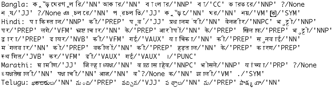
Figure 2.1: POS-Tagged Data from Four Indian Languages: Bangla, Hindi, Marathi, and Telugu
If the corpus is also segmented into sentences, it will have a tagged_sents() method that divides up the tagged words into sentences rather than presenting them as one big list. This will be useful when we come to developing automatic taggers, as they are trained and tested on lists of sentences, not words.
2.3 A Universal Part-of-Speech Tagset
Tagged corpora use many different conventions for tagging words. To help us get started, we will be looking at a simplified tagset (shown in 2.1).
| Tag | Meaning | English Examples |
|---|---|---|
| ADJ | adjective | new, good, high, special, big, local |
| ADP | adposition | on, of, at, with, by, into, under |
| ADV | adverb | really, already, still, early, now |
| CONJ | conjunction | and, or, but, if, while, although |
| DET | determiner, article | the, a, some, most, every, no, which |
| NOUN | noun | year, home, costs, time, Africa |
| NUM | numeral | twenty-four, fourth, 1991, 14:24 |
| PRT | particle | at, on, out, over per, that, up, with |
| PRON | pronoun | he, their, her, its, my, I, us |
| VERB | verb | is, say, told, given, playing, would |
| . | punctuation marks | . , ; ! |
| X | other | ersatz, esprit, dunno, gr8, univeristy |
Let's see which of these tags are the most common in the news category of the Brown corpus:
|
Note
Your Turn: Plot the above frequency distribution using tag_fd.plot(cumulative=True). What percentage of words are tagged using the first five tags of the above list?
We can use these tags to do powerful searches using a graphical POS-concordance tool nltk.app.concordance(). Use it to search for any combination of words and POS tags, e.g. N N N N, hit/VD, hit/VN, or the ADJ man.
2.4 Nouns
Nouns generally refer to people, places, things, or concepts, e.g.: woman, Scotland, book, intelligence. Nouns can appear after determiners and adjectives, and can be the subject or object of the verb, as shown in 2.2.
| Word | After a determiner | Subject of the verb |
|---|---|---|
| woman | the woman who I saw yesterday ... | the woman sat down |
| Scotland | the Scotland I remember as a child ... | Scotland has five million people |
| book | the book I bought yesterday ... | this book recounts the colonization of Australia |
| intelligence | the intelligence displayed by the child ... | Mary's intelligence impressed her teachers |
The simplified noun tags are N for common nouns like book, and NP for proper nouns like Scotland.
Let's inspect some tagged text to see what parts of speech occur before a noun, with the most frequent ones first. To begin with, we construct a list of bigrams whose members are themselves word-tag pairs such as (('The', 'DET'), ('Fulton', 'NP')) and (('Fulton', 'NP'), ('County', 'N')). Then we construct a FreqDist from the tag parts of the bigrams.
|
This confirms our assertion that nouns occur after determiners and adjectives, including numeral adjectives (tagged as NUM).
2.5 Verbs
Verbs are words that describe events and actions, e.g. fall, eat in 2.3. In the context of a sentence, verbs typically express a relation involving the referents of one or more noun phrases.
| Word | Simple | With modifiers and adjuncts (italicized) |
|---|---|---|
| fall | Rome fell | Dot com stocks suddenly fell like a stone |
| eat | Mice eat cheese | John ate the pizza with gusto |
What are the most common verbs in news text? Let's sort all the verbs by frequency:
|
Note that the items being counted in the frequency distribution are word-tag pairs. Since words and tags are paired, we can treat the word as a condition and the tag as an event, and initialize a conditional frequency distribution with a list of condition-event pairs. This lets us see a frequency-ordered list of tags given a word:
|
We can reverse the order of the pairs, so that the tags are the conditions, and the words are the events. Now we can see likely words for a given tag. We will do this for the WSJ tagset rather than the universal tagset:
|
To clarify the distinction between VBD (past tense) and VBN (past participle), let's find words which can be both VBD and VBN, and see some surrounding text:
|
In this case, we see that the past participle of kicked is preceded by a form of the auxiliary verb have. Is this generally true?
Note
Your Turn: Given the list of past participles produced by list(cfd2['VN']), try to collect a list of all the word-tag pairs that immediately precede items in that list.
2.6 Adjectives and Adverbs
Two other important word classes are adjectives and adverbs. Adjectives describe nouns, and can be used as modifiers (e.g. large in the large pizza), or in predicates (e.g. the pizza is large). English adjectives can have internal structure (e.g. fall+ing in the falling stocks). Adverbs modify verbs to specify the time, manner, place or direction of the event described by the verb (e.g. quickly in the stocks fell quickly). Adverbs may also modify adjectives (e.g. really in Mary's teacher was really nice).
English has several categories of closed class words in addition to prepositions, such as articles (also often called determiners) (e.g., the, a), modals (e.g., should, may), and personal pronouns (e.g., she, they). Each dictionary and grammar classifies these words differently.
Note
Your Turn: If you are uncertain about some of these parts of speech, study them using nltk.app.concordance(), or watch some of the Schoolhouse Rock! grammar videos available at YouTube, or consult the Further Reading section at the end of this chapter.
2.7 Unsimplified Tags
Let's find the most frequent nouns of each noun part-of-speech type. The program in 2.2 finds all tags starting with NN, and provides a few example words for each one. You will see that there are many variants of NN; the most important contain $ for possessive nouns, S for plural nouns (since plural nouns typically end in s) and P for proper nouns. In addition, most of the tags have suffix modifiers: -NC for citations, -HL for words in headlines and -TL for titles (a feature of Brown tags).
| ||
Example 2.2 (code_findtags.py): Figure 2.2: Program to Find the Most Frequent Noun Tags |
When we come to constructing part-of-speech taggers later in this chapter, we will use the unsimplified tags.
2.8 Exploring Tagged Corpora
Let's briefly return to the kinds of exploration of corpora we saw in previous chapters, this time exploiting POS tags.
Suppose we're studying the word often and want to see how it is used in text. We could ask to see the words that follow often
|
However, it's probably more instructive to use the tagged_words() method to look at the part-of-speech tag of the following words:
|
Notice that the most high-frequency parts of speech following often are verbs. Nouns never appear in this position (in this particular corpus).
Next, let's look at some larger context, and find words involving
particular sequences of tags and words (in this case "<Verb> to <Verb>").
In code-three-word-phrase we consider each three-word window in the sentence ![[1]](callouts/callout1.gif) ,
and check if they meet our criterion
,
and check if they meet our criterion ![[2]](callouts/callout2.gif) . If the tags
match, we print the corresponding words
. If the tags
match, we print the corresponding words ![[3]](callouts/callout3.gif) .
.
Example 2.3 (code_three_word_phrase.py): Figure 2.3: Searching for Three-Word Phrases Using POS Tags |
Finally, let's look for words that are highly ambiguous as to their part of speech tag. Understanding why such words are tagged as they are in each context can help us clarify the distinctions between the tags.
|
Note
Your Turn: Open the POS concordance tool nltk.app.concordance() and load the complete Brown Corpus (simplified tagset). Now pick some of the above words and see how the tag of the word correlates with the context of the word. E.g. search for near to see all forms mixed together, near/ADJ to see it used as an adjective, near N to see just those cases where a noun follows, and so forth. For a larger set of examples, modify the supplied code so that it lists words having three distinct tags.
3 Mapping Words to Properties Using Python Dictionaries
As we have seen, a tagged word of the form (word, tag) is an association between a word and a part-of-speech tag. Once we start doing part-of-speech tagging, we will be creating programs that assign a tag to a word, the tag which is most likely in a given context. We can think of this process as mapping from words to tags. The most natural way to store mappings in Python uses the so-called dictionary data type (also known as an associative array or hash array in other programming languages). In this section we look at dictionaries and see how they can represent a variety of language information, including parts of speech.
3.1 Indexing Lists vs Dictionaries
A text, as we have seen, is treated in Python as a list of words. An important property of lists is that we can "look up" a particular item by giving its index, e.g. text1[100]. Notice how we specify a number, and get back a word. We can think of a list as a simple kind of table, as shown in 3.1.
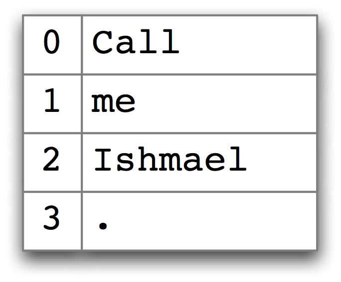
Figure 3.1: List Look-up: we access the contents of a Python list with the help of an integer index.
Contrast this situation with frequency distributions (3), where we specify a word, and get back a number, e.g. fdist['monstrous'], which tells us the number of times a given word has occurred in a text. Look-up using words is familiar to anyone who has used a dictionary. Some more examples are shown in 3.2.
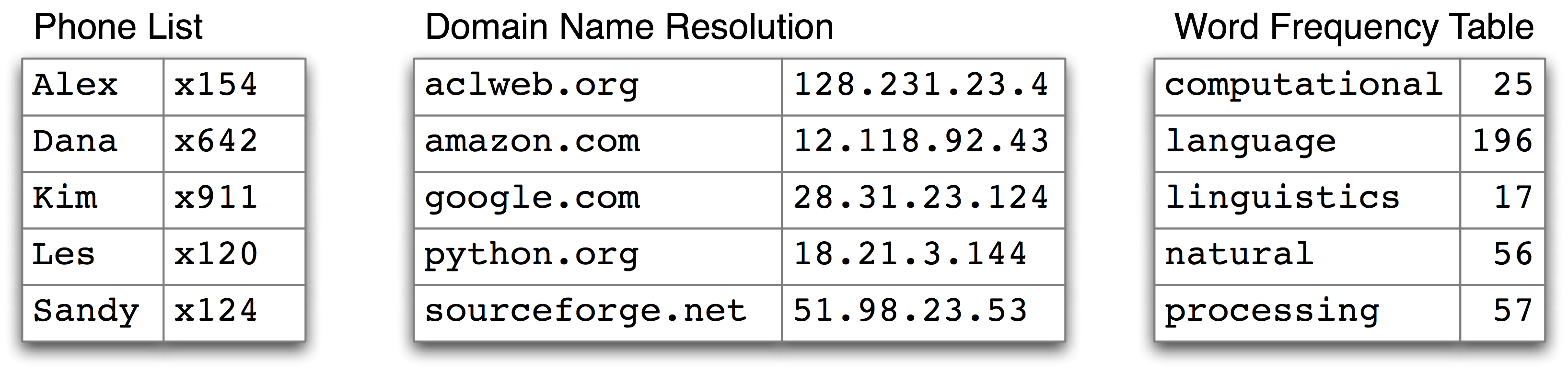
Figure 3.2: Dictionary Look-up: we access the entry of a dictionary using a key such as someone's name, a web domain, or an English word; other names for dictionary are map, hashmap, hash, and associative array.
In the case of a phonebook, we look up an entry using a name, and get back a number. When we type a domain name in a web browser, the computer looks this up to get back an IP address. A word frequency table allows us to look up a word and find its frequency in a text collection. In all these cases, we are mapping from names to numbers, rather than the other way around as with a list. In general, we would like to be able to map between arbitrary types of information. 3.1 lists a variety of linguistic objects, along with what they map.
| Linguistic Object | Maps From | Maps To |
|---|---|---|
| Document Index | Word | List of pages (where word is found) |
| Thesaurus | Word sense | List of synonyms |
| Dictionary | Headword | Entry (part-of-speech, sense definitions, etymology) |
| Comparative Wordlist | Gloss term | Cognates (list of words, one per language) |
| Morph Analyzer | Surface form | Morphological analysis (list of component morphemes) |
Most often, we are mapping from a "word" to some structured object. For example, a document index maps from a word (which we can represent as a string), to a list of pages (represented as a list of integers). In this section, we will see how to represent such mappings in Python.
3.2 Dictionaries in Python
Python provides a dictionary data type that can be used for mapping between arbitrary types. It is like a conventional dictionary, in that it gives you an efficient way to look things up. However, as we see from 3.1, it has a much wider range of uses.
To illustrate, we define pos to be an empty dictionary and then add four entries to it, specifying the part-of-speech of some words. We add entries to a dictionary using the familiar square bracket notation:
So, for example, says that
the part-of-speech of colorless is adjective, or more
specifically, that the key 'colorless'
is assigned the value 'ADJ' in dictionary pos.
When we inspect the value of pos we see
a set of key-value pairs. Once we have populated the dictionary
in this way, we can employ the keys to retrieve values:
|
Of course, we might accidentally use a key that hasn't been assigned a value.
|
This raises an important question. Unlike lists and strings, where we
can use len() to work out which integers will be legal indexes,
how do we work out the legal keys for a dictionary? If the dictionary
is not too big, we can simply inspect its contents by evaluating the
variable pos. As we saw above (line ), this gives
us the key-value pairs. Notice that they are not in the same order they
were originally entered; this is because dictionaries are not sequences
but mappings (cf. 3.2), and the keys are not inherently
ordered.
Alternatively, to just find the keys, we can convert the
dictionary to a list — or use
the dictionary in a context where a list is expected,
as the parameter of sorted() ,
or in a for loop .
|
Note
When you type list(pos) you might see a different order to the one shown above. If you want to see the keys in order, just sort them.
As well as iterating over all keys in the dictionary with a for loop, we can use the for loop as we did for printing lists:
|
Finally, the dictionary methods keys(), values() and
items() allow us to access the keys, values, and key-value pairs as separate lists.
We can even sort tuples , which orders them according to their first element
(and if the first elements are the same, it uses their second elements).
|
We want to be sure that when we look something up in a dictionary, we only get one value for each key. Now suppose we try to use a dictionary to store the fact that the word sleep can be used as both a verb and a noun:
|
Initially, pos['sleep'] is given the value 'V'. But this is immediately overwritten with the new value 'N'. In other words, there can only be one entry in the dictionary for 'sleep'. However, there is a way of storing multiple values in that entry: we use a list value, e.g. pos['sleep'] = ['N', 'V']. In fact, this is what we saw in 4 for the CMU Pronouncing Dictionary, which stores multiple pronunciations for a single word.
3.3 Defining Dictionaries
We can use the same key-value pair format to create a dictionary. There's a couple of ways to do this, and we will normally use the first:
|
Note that dictionary keys must be immutable types, such as strings and tuples. If we try to define a dictionary using a mutable key, we get a TypeError:
|
3.4 Default Dictionaries
If we try to access a key that is not in a dictionary, we get an error. However, its often useful if a dictionary can automatically create an entry for this new key and give it a default value, such as zero or the empty list. For this reason, a special kind of dictionary called a defaultdict is available. In order to use it, we have to supply a parameter which can be used to create the default value, e.g. int, float, str, list, dict, tuple.
|
Note
These default values are actually functions that convert other objects to the specified type (e.g. int("2"), list("2")). When they are called with no parameter — int(), list() — they return 0 and [] respectively.
The above examples specified the default value of a dictionary entry to
be the default value of a particular data type. However, we can specify
any default value we like, simply by providing the name of a function
that can be called with no arguments to create the required value.
Let's return to our part-of-speech example, and create a dictionary
whose default value for any entry is 'N' .
When we access a non-existent entry ,
it is automatically added to the dictionary .
|
Note
The above example used a lambda expression, introduced in 4.4. This lambda expression specifies no parameters, so we call it using parentheses with no arguments. Thus, the definitions of f and g below are equivalent:
|
Let's see how default dictionaries could be used in a more substantial language processing task. Many language processing tasks — including tagging — struggle to correctly process the hapaxes of a text. They can perform better with a fixed vocabulary and a guarantee that no new words will appear. We can preprocess a text to replace low-frequency words with a special "out of vocabulary" token UNK, with the help of a default dictionary. (Can you work out how to do this without reading on?)
We need to create a default dictionary that maps each word to its replacement. The most frequent n words will be mapped to themselves. Everything else will be mapped to UNK.
|
3.5 Incrementally Updating a Dictionary
We can employ dictionaries to count occurrences, emulating the method for tallying words shown in fig-tally. We begin by initializing an empty defaultdict, then process each part-of-speech tag in the text. If the tag hasn't been seen before, it will have a zero count by default. Each time we encounter a tag, we increment its count using the += operator.
| ||
Example 3.3 (code_dictionary.py): Figure 3.3: Incrementally Updating a Dictionary, and Sorting by Value |
The listing in 3.3 illustrates an important idiom for sorting a dictionary by its values, to show words in decreasing order of frequency. The first parameter of sorted() is the items to sort, a list of tuples consisting of a POS tag and a frequency. The second parameter specifies the sort key using a function itemgetter(). In general, itemgetter(n) returns a function that can be called on some other sequence object to obtain the nth element, e.g.:
|
The last parameter of sorted() specifies that the items should be returned in reverse order, i.e. decreasing values of frequency.
There's a second useful programming idiom at the beginning of 3.3, where we initialize a defaultdict and then use a for loop to update its values. Here's a schematic version:
Here's another instance of this pattern, where we index words according to their last two letters:
|
The following example uses the same pattern to create an anagram dictionary. (You might experiment with the third line to get an idea of why this program works.)
|
Since accumulating words like this is such a common task, NLTK provides a more convenient way of creating a defaultdict(list), in the form of nltk.Index().
|
Note
nltk.Index is a defaultdict(list) with extra support for initialization. Similarly, nltk.FreqDist is essentially a defaultdict(int) with extra support for initialization (along with sorting and plotting methods).
3.6 Complex Keys and Values
We can use default dictionaries with complex keys and values. Let's study the range of possible tags for a word, given the word itself, and the tag of the previous word. We will see how this information can be used by a POS tagger.
|
This example uses a dictionary whose default value for an entry
is a dictionary (whose default value is int(), i.e. zero).
Notice how we iterated over the bigrams of the tagged
corpus, processing a pair of word-tag pairs for each iteration .
Each time through the loop we updated our pos dictionary's
entry for (t1, w2), a tag and its following word .
When we look up an item in pos we must specify a compound key ,
and we get back a dictionary object.
A POS tagger could use such information to decide that the
word right, when preceded by a determiner, should be tagged as ADJ.
3.7 Inverting a Dictionary
Dictionaries support efficient lookup, so long as you want to get the value for any key. If d is a dictionary and k is a key, we type d[k] and immediately obtain the value. Finding a key given a value is slower and more cumbersome:
|
If we expect to do this kind of "reverse lookup" often, it helps to construct a dictionary that maps values to keys. In the case that no two keys have the same value, this is an easy thing to do. We just get all the key-value pairs in the dictionary, and create a new dictionary of value-key pairs. The next example also illustrates another way of initializing a dictionary pos with key-value pairs.
|
Let's first make our part-of-speech dictionary a bit more realistic and add some more words to pos using the dictionary update() method, to create the situation where multiple keys have the same value. Then the technique just shown for reverse lookup will no longer work (why not?). Instead, we have to use append() to accumulate the words for each part-of-speech, as follows:
|
Now we have inverted the pos dictionary, and can look up any part-of-speech and find all words having that part-of-speech. We can do the same thing even more simply using NLTK's support for indexing as follows:
|
A summary of Python's dictionary methods is given in 3.2.
| Example | Description |
|---|---|
| d = {} | create an empty dictionary and assign it to d |
| d[key] = value | assign a value to a given dictionary key |
| d.keys() | the list of keys of the dictionary |
| list(d) | the list of keys of the dictionary |
| sorted(d) | the keys of the dictionary, sorted |
| key in d | test whether a particular key is in the dictionary |
| for key in d | iterate over the keys of the dictionary |
| d.values() | the list of values in the dictionary |
| dict([(k1,v1), (k2,v2), ...]) | create a dictionary from a list of key-value pairs |
| d1.update(d2) | add all items from d2 to d1 |
| defaultdict(int) | a dictionary whose default value is zero |
4 Automatic Tagging
In the rest of this chapter we will explore various ways to automatically add part-of-speech tags to text. We will see that the tag of a word depends on the word and its context within a sentence. For this reason, we will be working with data at the level of (tagged) sentences rather than words. We'll begin by loading the data we will be using.
|
4.1 The Default Tagger
The simplest possible tagger assigns the same tag to each token. This may seem to be a rather banal step, but it establishes an important baseline for tagger performance. In order to get the best result, we tag each word with the most likely tag. Let's find out which tag is most likely (now using the unsimplified tagset):
|
Now we can create a tagger that tags everything as NN.
|
Unsurprisingly, this method performs rather poorly. On a typical corpus, it will tag only about an eighth of the tokens correctly, as we see below:
|
Default taggers assign their tag to every single word, even words that have never been encountered before. As it happens, once we have processed several thousand words of English text, most new words will be nouns. As we will see, this means that default taggers can help to improve the robustness of a language processing system. We will return to them shortly.
4.2 The Regular Expression Tagger
The regular expression tagger assigns tags to tokens on the basis of matching patterns. For instance, we might guess that any word ending in ed is the past participle of a verb, and any word ending with 's is a possessive noun. We can express these as a list of regular expressions:
|
Note that these are processed in order, and the first one that matches is applied. Now we can set up a tagger and use it to tag a sentence. Now its right about a fifth of the time.
|
The final regular expression «.*» is a catch-all that tags everything as a noun. This is equivalent to the default tagger (only much less efficient). Instead of re-specifying this as part of the regular expression tagger, is there a way to combine this tagger with the default tagger? We will see how to do this shortly.
Note
Your Turn: See if you can come up with patterns to improve the performance of the above regular expression tagger. (Note that 1 describes a way to partially automate such work.)
4.3 The Lookup Tagger
A lot of high-frequency words do not have the NN tag. Let's find the hundred most frequent words and store their most likely tag. We can then use this information as the model for a "lookup tagger" (an NLTK UnigramTagger):
|
It should come as no surprise by now that simply knowing the tags for the 100 most frequent words enables us to tag a large fraction of tokens correctly (nearly half in fact). Let's see what it does on some untagged input text:
|
Many words have been assigned a tag of None, because they were not among the 100 most frequent words. In these cases we would like to assign the default tag of NN. In other words, we want to use the lookup table first, and if it is unable to assign a tag, then use the default tagger, a process known as backoff (5). We do this by specifying one tagger as a parameter to the other, as shown below. Now the lookup tagger will only store word-tag pairs for words other than nouns, and whenever it cannot assign a tag to a word it will invoke the default tagger.
|
Let's put all this together and write a program to create and evaluate lookup taggers having a range of sizes, in 4.1.
| ||
| ||
Example 4.1 (code_baseline_tagger.py): Figure 4.1: Lookup Tagger Performance with Varying Model Size |
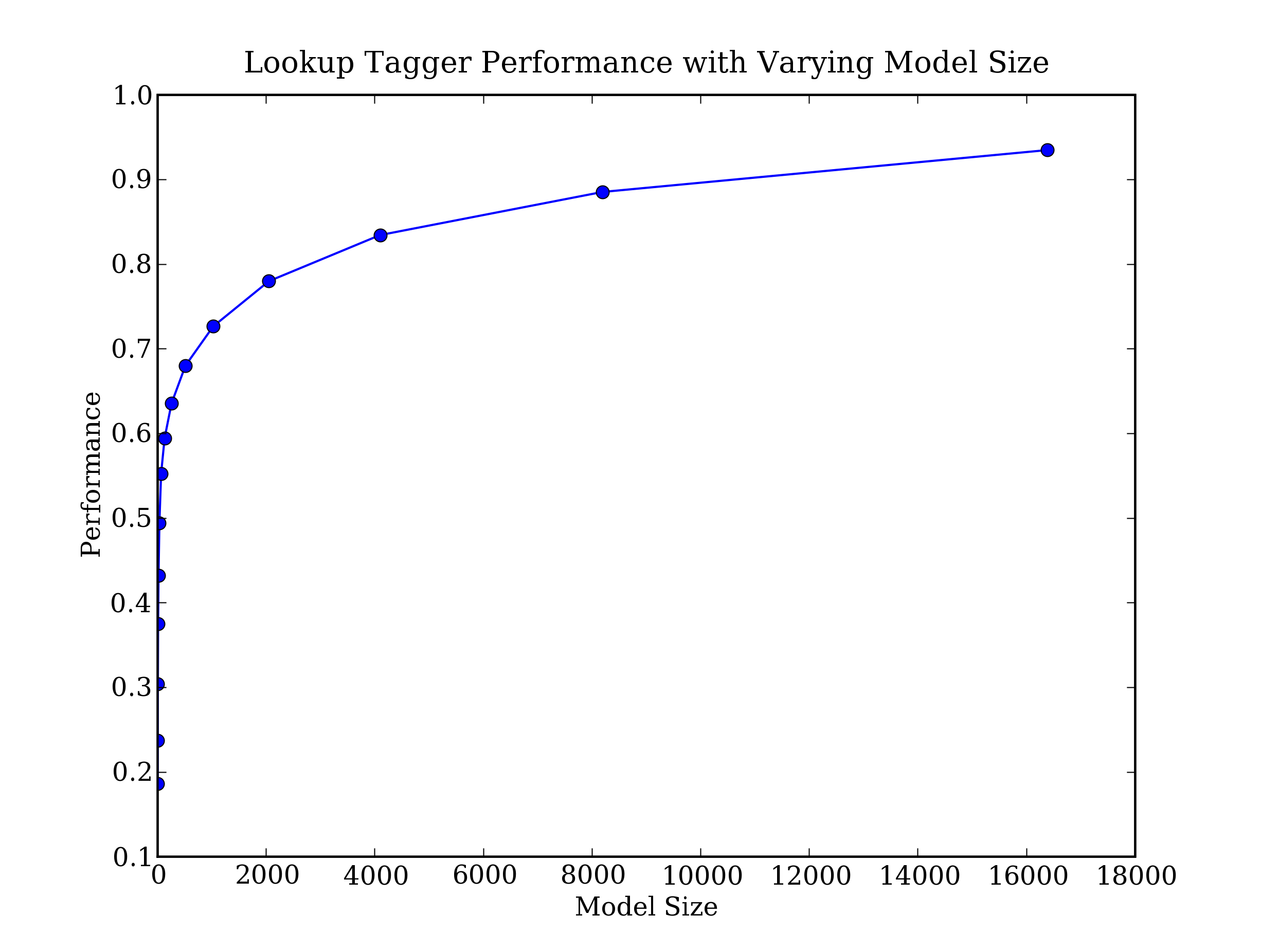
Figure 4.2: Lookup Tagger
Observe that performance initially increases rapidly as the model size grows, eventually reaching a plateau, when large increases in model size yield little improvement in performance. (This example used the pylab plotting package, discussed in 4.8.)
4.4 Evaluation
In the above examples, you will have noticed an emphasis on accuracy scores. In fact, evaluating the performance of such tools is a central theme in NLP. Recall the processing pipeline in fig-sds; any errors in the output of one module are greatly multiplied in the downstream modules.
We evaluate the performance of a tagger relative to the tags a human expert would assign. Since we don't usually have access to an expert and impartial human judge, we make do instead with gold standard test data. This is a corpus which has been manually annotated and which is accepted as a standard against which the guesses of an automatic system are assessed. The tagger is regarded as being correct if the tag it guesses for a given word is the same as the gold standard tag.
Of course, the humans who designed and carried out the original gold standard annotation were only human. Further analysis might show mistakes in the gold standard, or may eventually lead to a revised tagset and more elaborate guidelines. Nevertheless, the gold standard is by definition "correct" as far as the evaluation of an automatic tagger is concerned.
Note
Developing an annotated corpus is a major undertaking. Apart from the data, it generates sophisticated tools, documentation, and practices for ensuring high quality annotation. The tagsets and other coding schemes inevitably depend on some theoretical position that is not shared by all, however corpus creators often go to great lengths to make their work as theory-neutral as possible in order to maximize the usefulness of their work. We will discuss the challenges of creating a corpus in 11..
5 N-Gram Tagging
5.1 Unigram Tagging
Unigram taggers are based on a simple statistical algorithm: for each token, assign the tag that is most likely for that particular token. For example, it will assign the tag JJ to any occurrence of the word frequent, since frequent is used as an adjective (e.g. a frequent word) more often than it is used as a verb (e.g. I frequent this cafe). A unigram tagger behaves just like a lookup tagger (4), except there is a more convenient technique for setting it up, called training. In the following code sample, we train a unigram tagger, use it to tag a sentence, then evaluate:
|
We train a UnigramTagger by specifying tagged sentence data as a parameter when we initialize the tagger. The training process involves inspecting the tag of each word and storing the most likely tag for any word in a dictionary, stored inside the tagger.
5.2 Separating the Training and Testing Data
Now that we are training a tagger on some data, we must be careful not to test it on the same data, as we did in the above example. A tagger that simply memorized its training data and made no attempt to construct a general model would get a perfect score, but would also be useless for tagging new text. Instead, we should split the data, training on 90% and testing on the remaining 10%:
|
Although the score is worse, we now have a better picture of the usefulness of this tagger, i.e. its performance on previously unseen text.
5.3 General N-Gram Tagging
When we perform a language processing task based on unigrams, we are using one item of context. In the case of tagging, we only consider the current token, in isolation from any larger context. Given such a model, the best we can do is tag each word with its a priori most likely tag. This means we would tag a word such as wind with the same tag, regardless of whether it appears in the context the wind or to wind.
An n-gram tagger is a generalization of a unigram tagger whose context is the current word together with the part-of-speech tags of the n-1 preceding tokens, as shown in 5.1. The tag to be chosen, tn, is circled, and the context is shaded in grey. In the example of an n-gram tagger shown in 5.1, we have n=3; that is, we consider the tags of the two preceding words in addition to the current word. An n-gram tagger picks the tag that is most likely in the given context.
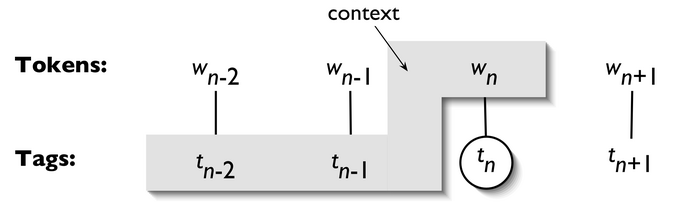
Figure 5.1: Tagger Context
Note
A 1-gram tagger is another term for a unigram tagger: i.e., the context used to tag a token is just the text of the token itself. 2-gram taggers are also called bigram taggers, and 3-gram taggers are called trigram taggers.
The NgramTagger class uses a tagged training corpus to determine which part-of-speech tag is most likely for each context. Here we see a special case of an n-gram tagger, namely a bigram tagger. First we train it, then use it to tag untagged sentences:
|
Notice that the bigram tagger manages to tag every word in a sentence it saw during training, but does badly on an unseen sentence. As soon as it encounters a new word (i.e., 13.5), it is unable to assign a tag. It cannot tag the following word (i.e., million) even if it was seen during training, simply because it never saw it during training with a None tag on the previous word. Consequently, the tagger fails to tag the rest of the sentence. Its overall accuracy score is very low:
|
As n gets larger, the specificity of the contexts increases, as does the chance that the data we wish to tag contains contexts that were not present in the training data. This is known as the sparse data problem, and is quite pervasive in NLP. As a consequence, there is a trade-off between the accuracy and the coverage of our results (and this is related to the precision/recall trade-off in information retrieval).
Caution!
n-gram taggers should not consider context that crosses a sentence boundary. Accordingly, NLTK taggers are designed to work with lists of sentences, where each sentence is a list of words. At the start of a sentence, tn-1 and preceding tags are set to None.
5.4 Combining Taggers
One way to address the trade-off between accuracy and coverage is to use the more accurate algorithms when we can, but to fall back on algorithms with wider coverage when necessary. For example, we could combine the results of a bigram tagger, a unigram tagger, and a default tagger, as follows:
- Try tagging the token with the bigram tagger.
- If the bigram tagger is unable to find a tag for the token, try the unigram tagger.
- If the unigram tagger is also unable to find a tag, use a default tagger.
Most NLTK taggers permit a backoff-tagger to be specified. The backoff-tagger may itself have a backoff tagger:
|
Note
Your Turn: Extend the above example by defining a TrigramTagger called t3, which backs off to t2.
Note that we specify the backoff tagger when the tagger is initialized so that training can take advantage of the backoff tagger. Thus, if the bigram tagger would assign the same tag as its unigram backoff tagger in a certain context, the bigram tagger discards the training instance. This keeps the bigram tagger model as small as possible. We can further specify that a tagger needs to see more than one instance of a context in order to retain it, e.g. nltk.BigramTagger(sents, cutoff=2, backoff=t1) will discard contexts that have only been seen once or twice.
5.5 Tagging Unknown Words
Our approach to tagging unknown words still uses backoff to a regular-expression tagger or a default tagger. These are unable to make use of context. Thus, if our tagger encountered the word blog, not seen during training, it would assign it the same tag, regardless of whether this word appeared in the context the blog or to blog. How can we do better with these unknown words, or out-of-vocabulary items?
A useful method to tag unknown words based on context is to limit the vocabulary of a tagger to the most frequent n words, and to replace every other word with a special word UNK using the method shown in 3. During training, a unigram tagger will probably learn that UNK is usually a noun. However, the n-gram taggers will detect contexts in which it has some other tag. For example, if the preceding word is to (tagged TO), then UNK will probably be tagged as a verb.
5.6 Storing Taggers
Training a tagger on a large corpus may take a significant time. Instead of training a tagger every time we need one, it is convenient to save a trained tagger in a file for later re-use. Let's save our tagger t2 to a file t2.pkl.
|
Now, in a separate Python process, we can load our saved tagger.
|
Now let's check that it can be used for tagging.
|
5.7 Performance Limitations
What is the upper limit to the performance of an n-gram tagger? Consider the case of a trigram tagger. How many cases of part-of-speech ambiguity does it encounter? We can determine the answer to this question empirically:
|
Thus, one out of twenty trigrams is ambiguous [EXAMPLES]. Given the current word and the previous two tags, in 5% of cases there is more than one tag that could be legitimately assigned to the current word according to the training data. Assuming we always pick the most likely tag in such ambiguous contexts, we can derive a lower bound on the performance of a trigram tagger.
Another way to investigate the performance of a tagger is to study its mistakes. Some tags may be harder than others to assign, and it might be possible to treat them specially by pre- or post-processing the data. A convenient way to look at tagging errors is the confusion matrix. It charts expected tags (the gold standard) against actual tags generated by a tagger:
|
Based on such analysis we may decide to modify the tagset. Perhaps a distinction between tags that is difficult to make can be dropped, since it is not important in the context of some larger processing task.
Another way to analyze the performance bound on a tagger comes from the less than 100% agreement between human annotators. [MORE]
In general, observe that the tagging process collapses distinctions: e.g. lexical identity is usually lost when all personal pronouns are tagged PRP. At the same time, the tagging process introduces new distinctions and removes ambiguities: e.g. deal tagged as VB or NN. This characteristic of collapsing certain distinctions and introducing new distinctions is an important feature of tagging which facilitates classification and prediction. When we introduce finer distinctions in a tagset, an n-gram tagger gets more detailed information about the left-context when it is deciding what tag to assign to a particular word. However, the tagger simultaneously has to do more work to classify the current token, simply because there are more tags to choose from. Conversely, with fewer distinctions (as with the simplified tagset), the tagger has less information about context, and it has a smaller range of choices in classifying the current token.
We have seen that ambiguity in the training data leads to an upper limit in tagger performance. Sometimes more context will resolve the ambiguity. In other cases however, as noted by (Church, Young, & Bloothooft, 1996), the ambiguity can only be resolved with reference to syntax, or to world knowledge. Despite these imperfections, part-of-speech tagging has played a central role in the rise of statistical approaches to natural language processing. In the early 1990s, the surprising accuracy of statistical taggers was a striking demonstration that it was possible to solve one small part of the language understanding problem, namely part-of-speech disambiguation, without reference to deeper sources of linguistic knowledge. Can this idea be pushed further? In 7., we shall see that it can.
6 Transformation-Based Tagging
A potential issue with n-gram taggers is the size of their n-gram table (or language model). If tagging is to be employed in a variety of language technologies deployed on mobile computing devices, it is important to strike a balance between model size and tagger performance. An n-gram tagger with backoff may store trigram and bigram tables, large sparse arrays which may have hundreds of millions of entries.
A second issue concerns context. The only information an n-gram tagger considers from prior context is tags, even though words themselves might be a useful source of information. It is simply impractical for n-gram models to be conditioned on the identities of words in the context. In this section we examine Brill tagging, an inductive tagging method which performs very well using models that are only a tiny fraction of the size of n-gram taggers.
Brill tagging is a kind of transformation-based learning, named after its inventor. The general idea is very simple: guess the tag of each word, then go back and fix the mistakes. In this way, a Brill tagger successively transforms a bad tagging of a text into a better one. As with n-gram tagging, this is a supervised learning method, since we need annotated training data to figure out whether the tagger's guess is a mistake or not. However, unlike n-gram tagging, it does not count observations but compiles a list of transformational correction rules.
The process of Brill tagging is usually explained by analogy with painting. Suppose we were painting a tree, with all its details of boughs, branches, twigs and leaves, against a uniform sky-blue background. Instead of painting the tree first then trying to paint blue in the gaps, it is simpler to paint the whole canvas blue, then "correct" the tree section by over-painting the blue background. In the same fashion we might paint the trunk a uniform brown before going back to over-paint further details with even finer brushes. Brill tagging uses the same idea: begin with broad brush strokes then fix up the details, with successively finer changes. Let's look at an example involving the following sentence:
| (1) | The President said he will ask Congress to increase grants to states for vocational rehabilitation |
We will examine the operation of two rules: (a) Replace NN with VB when the previous word is TO; (b) Replace TO with IN when the next tag is NNS. 6.1 illustrates this process, first tagging with the unigram tagger, then applying the rules to fix the errors.
| Phrase | to | increase | grants | to | states | for | vocational | rehabilitation |
| Unigram | TO | NN | NNS | TO | NNS | IN | JJ | NN |
| Rule 1 | VB | |||||||
| Rule 2 | IN | |||||||
| Output | TO | VB | NNS | IN | NNS | IN | JJ | NN |
| Gold | TO | VB | NNS | IN | NNS | IN | JJ | NN |
In this table we see two rules. All such rules are generated from a template of the following form: "replace T1 with T2 in the context C". Typical contexts are the identity or the tag of the preceding or following word, or the appearance of a specific tag within 2-3 words of the current word. During its training phase, the tagger guesses values for T1, T2 and C, to create thousands of candidate rules. Each rule is scored according to its net benefit: the number of incorrect tags that it corrects, less the number of correct tags it incorrectly modifies.
Brill taggers have another interesting property: the rules are linguistically interpretable. Compare this with the n-gram taggers, which employ a potentially massive table of n-grams. We cannot learn much from direct inspection of such a table, in comparison to the rules learned by the Brill tagger. 6.1 demonstrates NLTK's Brill tagger.
| ||
Example 6.1 (code_brill_demo.py): Figure 6.1: Brill Tagger Demonstration: the tagger has a collection of templates of the form X -> Y if the preceding word is Z; the variables in these templates are instantiated to particular words and tags to create "rules"; the score for a rule is the number of broken examples it corrects minus the number of correct cases it breaks; apart from training a tagger, the demonstration displays residual errors. |
7 How to Determine the Category of a Word
Now that we have examined word classes in detail, we turn to a more basic question: how do we decide what category a word belongs to in the first place? In general, linguists use morphological, syntactic, and semantic clues to determine the category of a word.
7.1 Morphological Clues
The internal structure of a word may give useful clues as to the word's category. For example, -ness is a suffix that combines with an adjective to produce a noun, e.g. happy → happiness, ill → illness. So if we encounter a word that ends in -ness, this is very likely to be a noun. Similarly, -ment is a suffix that combines with some verbs to produce a noun, e.g. govern → government and establish → establishment.
English verbs can also be morphologically complex. For instance, the present participle of a verb ends in -ing, and expresses the idea of ongoing, incomplete action (e.g. falling, eating). The -ing suffix also appears on nouns derived from verbs, e.g. the falling of the leaves (this is known as the gerund).
7.2 Syntactic Clues
Another source of information is the typical contexts in which a word can occur. For example, assume that we have already determined the category of nouns. Then we might say that a syntactic criterion for an adjective in English is that it can occur immediately before a noun, or immediately following the words be or very. According to these tests, near should be categorized as an adjective:
| (2) |
|
7.3 Semantic Clues
Finally, the meaning of a word is a useful clue as to its lexical category. For example, the best-known definition of a noun is semantic: "the name of a person, place or thing". Within modern linguistics, semantic criteria for word classes are treated with suspicion, mainly because they are hard to formalize. Nevertheless, semantic criteria underpin many of our intuitions about word classes, and enable us to make a good guess about the categorization of words in languages that we are unfamiliar with. For example, if all we know about the Dutch word verjaardag is that it means the same as the English word birthday, then we can guess that verjaardag is a noun in Dutch. However, some care is needed: although we might translate zij is vandaag jarig as it's her birthday today, the word jarig is in fact an adjective in Dutch, and has no exact equivalent in English.
7.4 New Words
All languages acquire new lexical items. A list of words recently added to the Oxford Dictionary of English includes cyberslacker, fatoush, blamestorm, SARS, cantopop, bupkis, noughties, muggle, and robata. Notice that all these new words are nouns, and this is reflected in calling nouns an open class. By contrast, prepositions are regarded as a closed class. That is, there is a limited set of words belonging to the class (e.g., above, along, at, below, beside, between, during, for, from, in, near, on, outside, over, past, through, towards, under, up, with), and membership of the set only changes very gradually over time.
7.5 Morphology in Part of Speech Tagsets
Common tagsets often capture some morpho-syntactic information; that is, information about the kind of morphological markings that words receive by virtue of their syntactic role. Consider, for example, the selection of distinct grammatical forms of the word go illustrated in the following sentences:
| (3) |
|
Each of these forms — go, goes, gone, and went — is morphologically distinct from the others. Consider the form, goes. This occurs in a restricted set of grammatical contexts, and requires a third person singular subject. Thus, the following sentences are ungrammatical.
| (4) |
|
By contrast, gone is the past participle form; it is required after have (and cannot be replaced in this context by goes), and cannot occur as the main verb of a clause.
| (5) |
|
We can easily imagine a tagset in which the four distinct grammatical forms just discussed were all tagged as VB. Although this would be adequate for some purposes, a more fine-grained tagset provides useful information about these forms that can help other processors that try to detect patterns in tag sequences. The Brown tagset captures these distinctions, as summarized in 7.1.
| Form | Category | Tag |
|---|---|---|
| go | base | VB |
| goes | 3rd singular present | VBZ |
| gone | past participle | VBN |
| going | gerund | VBG |
| went | simple past | VBD |
In addition to this set of verb tags, the various forms of the verb to be have special tags: be/BE, being/BEG, am/BEM, are/BER, is/BEZ, been/BEN, were/BED and was/BEDZ (plus extra tags for negative forms of the verb). All told, this fine-grained tagging of verbs means that an automatic tagger that uses this tagset is effectively carrying out a limited amount of morphological analysis.
Most part-of-speech tagsets make use of the same basic categories, such as noun, verb, adjective, and preposition. However, tagsets differ both in how finely they divide words into categories, and in how they define their categories. For example, is might be tagged simply as a verb in one tagset; but as a distinct form of the lexeme be in another tagset (as in the Brown Corpus). This variation in tagsets is unavoidable, since part-of-speech tags are used in different ways for different tasks. In other words, there is no one 'right way' to assign tags, only more or less useful ways depending on one's goals.
8 Summary
- Words can be grouped into classes, such as nouns, verbs, adjectives, and adverbs. These classes are known as lexical categories or parts of speech. Parts of speech are assigned short labels, or tags, such as NN, VB,
- The process of automatically assigning parts of speech to words in text is called part-of-speech tagging, POS tagging, or just tagging.
- Automatic tagging is an important step in the NLP pipeline, and is useful in a variety of situations including: predicting the behavior of previously unseen words, analyzing word usage in corpora, and text-to-speech systems.
- Some linguistic corpora, such as the Brown Corpus, have been POS tagged.
- A variety of tagging methods are possible, e.g. default tagger, regular expression tagger, unigram tagger and n-gram taggers. These can be combined using a technique known as backoff.
- Taggers can be trained and evaluated using tagged corpora.
- Backoff is a method for combining models: when a more specialized model (such as a bigram tagger) cannot assign a tag in a given context, we backoff to a more general model (such as a unigram tagger).
- Part-of-speech tagging is an important, early example of a sequence classification task in NLP: a classification decision at any one point in the sequence makes use of words and tags in the local context.
- A dictionary is used to map between arbitrary types of information, such as a string and a number: freq['cat'] = 12. We create dictionaries using the brace notation: pos = {}, pos = {'furiously': 'adv', 'ideas': 'n', 'colorless': 'adj'}.
- N-gram taggers can be defined for large values of n, but once n is larger than 3 we usually encounter the sparse data problem; even with a large quantity of training data we only see a tiny fraction of possible contexts.
- Transformation-based tagging involves learning a series of repair rules of the form "change tag s to tag t in context c", where each rule fixes mistakes and possibly introduces a (smaller) number of errors.
9 Further Reading
Extra materials for this chapter are posted at http://nltk.org/, including links to freely available resources on the web. For more examples of tagging with NLTK, please see the Tagging HOWTO at http://nltk.org/howto. Chapters 4 and 5 of (Jurafsky & Martin, 2008) contain more advanced material on n-grams and part-of-speech tagging. The "Universal Tagset" is described by (Petrov, Das, & McDonald, 2012). Other approaches to tagging involve machine learning methods (chap-data-intensive). In 7. we will see a generalization of tagging called chunking in which a contiguous sequence of words is assigned a single tag.
For tagset documentation, see nltk.help.upenn_tagset() and nltk.help.brown_tagset(). Lexical categories are introduced in linguistics textbooks, including those listed in 1..
There are many other kinds of tagging. Words can be tagged with directives to a speech synthesizer, indicating which words should be emphasized. Words can be tagged with sense numbers, indicating which sense of the word was used. Words can also be tagged with morphological features. Examples of each of these kinds of tags are shown below. For space reasons, we only show the tag for a single word. Note also that the first two examples use XML-style tags, where elements in angle brackets enclose the word that is tagged.
- Speech Synthesis Markup Language (W3C SSML): That is a <emphasis>big</emphasis> car!
- SemCor: Brown Corpus tagged with WordNet senses: Space in any <wf pos="NN" lemma="form" wnsn="4">form</wf> is completely measured by the three dimensions. (Wordnet form/nn sense 4: "shape, form, configuration, contour, conformation")
- Morphological tagging, from the Turin University Italian Treebank: E' italiano , come progetto e realizzazione , il primo (PRIMO ADJ ORDIN M SING) porto turistico dell' Albania .
Note that tagging is also performed at higher levels. Here is an example of dialogue act tagging, from the NPS Chat Corpus (Forsyth & Martell, 2007) included with NLTK. Each turn of the dialogue is categorized as to its communicative function:
Statement  User117 Dude..., I wanted some of that
ynQuestion User120 m I missing something?
Bye        User117 I'm gonna go fix food, I'll be back later.
System     User122 JOIN
System     User2   slaps User122 around a bit with a large trout.
Statement  User121 18/m pm me if u tryin to chat
10 Exercises
- ☼ Search the web for "spoof newspaper headlines", to find such gems as: British Left Waffles on Falkland Islands, and Juvenile Court to Try Shooting Defendant. Manually tag these headlines to see if knowledge of the part-of-speech tags removes the ambiguity.
- ☼ Working with someone else, take turns to pick a word that can be either a noun or a verb (e.g. contest); the opponent has to predict which one is likely to be the most frequent in the Brown corpus; check the opponent's prediction, and tally the score over several turns.
- ☼ Tokenize and tag the following sentence: They wind back the clock, while we chase after the wind. What different pronunciations and parts of speech are involved?
- ☼ Review the mappings in 3.1. Discuss any other examples of mappings you can think of. What type of information do they map from and to?
- ☼ Using the Python interpreter in interactive mode, experiment with the dictionary examples in this chapter. Create a dictionary d, and add some entries. What happens if you try to access a non-existent entry, e.g. d['xyz']?
- ☼ Try deleting an element from a dictionary d, using the syntax del d['abc']. Check that the item was deleted.
- ☼ Create two dictionaries, d1 and d2, and add some entries to each. Now issue the command d1.update(d2). What did this do? What might it be useful for?
- ☼ Create a dictionary e, to represent a single lexical entry for some word of your choice. Define keys like headword, part-of-speech, sense, and example, and assign them suitable values.
- ☼ Satisfy yourself that there are restrictions on the distribution of go and went, in the sense that they cannot be freely interchanged in the kinds of contexts illustrated in (3d) in 7.
- ☼ Train a unigram tagger and run it on some new text. Observe that some words are not assigned a tag. Why not?
- ☼ Learn about the affix tagger (type help(nltk.AffixTagger)). Train an affix tagger and run it on some new text. Experiment with different settings for the affix length and the minimum word length. Discuss your findings.
- ☼ Train a bigram tagger with no backoff tagger, and run it on some of the training data. Next, run it on some new data. What happens to the performance of the tagger? Why?
- ☼ We can use a dictionary to specify the values to be substituted into a formatting string. Read Python's library documentation for formatting strings http://docs.python.org/lib/typesseq-strings.html and use this method to display today's date in two different formats.
- ◑ Use sorted() and set() to get a sorted list of tags used in the Brown corpus, removing duplicates.
- ◑ Write programs to process the Brown Corpus and find answers to the following
questions:
- Which nouns are more common in their plural form, rather than their singular form? (Only consider regular plurals, formed with the -s suffix.)
- Which word has the greatest number of distinct tags. What are they, and what do they represent?
- List tags in order of decreasing frequency. What do the 20 most frequent tags represent?
- Which tags are nouns most commonly found after? What do these tags represent?
- ◑ Explore the following issues that arise in connection with the lookup tagger:
- What happens to the tagger performance for the various model sizes when a backoff tagger is omitted?
- Consider the curve in 4.2; suggest a good size for a lookup tagger that balances memory and performance. Can you come up with scenarios where it would be preferable to minimize memory usage, or to maximize performance with no regard for memory usage?
- ◑ What is the upper limit of performance for a lookup tagger, assuming no limit to the size of its table? (Hint: write a program to work out what percentage of tokens of a word are assigned the most likely tag for that word, on average.)
- ◑ Generate some statistics for tagged data to answer the following questions:
- What proportion of word types are always assigned the same part-of-speech tag?
- How many words are ambiguous, in the sense that they appear with at least two tags?
- What percentage of word tokens in the Brown Corpus involve these ambiguous words?
- ◑ The evaluate() method works out how accurately
the tagger performs on this text. For example, if the supplied tagged text
was [('the', 'DT'), ('dog', 'NN')] and the tagger produced the output
[('the', 'NN'), ('dog', 'NN')], then the score would be 0.5.
Let's try to figure out how the evaluation method works:
- A tagger t takes a list of words as input, and produces a list of tagged words as output. However, t.evaluate() is given correctly tagged text as its only parameter. What must it do with this input before performing the tagging?
- Once the tagger has created newly tagged text, how might the evaluate() method go about comparing it with the original tagged text and computing the accuracy score?
- Now examine the source code to see how the method is implemented. Inspect nltk.tag.api.__file__ to discover the location of the source code, and open this file using an editor (be sure to use the api.py file and not the compiled api.pyc binary file).
- ◑ Write code to search the Brown Corpus for particular words and phrases
according to tags, to answer the following questions:
- Produce an alphabetically sorted list of the distinct words tagged as MD.
- Identify words that can be plural nouns or third person singular verbs (e.g. deals, flies).
- Identify three-word prepositional phrases of the form IN + DET + NN (eg. in the lab).
- What is the ratio of masculine to feminine pronouns?
- ◑ In 3.1 we saw a table involving frequency counts for the verbs adore, love, like, prefer and preceding qualifiers absolutely and definitely. Investigate the full range of adverbs that appear before these four verbs.
- ◑ We defined the regexp_tagger that can be used as a fall-back tagger for unknown words. This tagger only checks for cardinal numbers. By testing for particular prefix or suffix strings, it should be possible to guess other tags. For example, we could tag any word that ends with -s as a plural noun. Define a regular expression tagger (using RegexpTagger()) that tests for at least five other patterns in the spelling of words. (Use inline documentation to explain the rules.)
- ◑ Consider the regular expression tagger developed in the exercises in the previous section. Evaluate the tagger using its accuracy() method, and try to come up with ways to improve its performance. Discuss your findings. How does objective evaluation help in the development process?
- ◑ How serious is the sparse data problem? Investigate the performance of n-gram taggers as n increases from 1 to 6. Tabulate the accuracy score. Estimate the training data required for these taggers, assuming a vocabulary size of 105 and a tagset size of 102.
- ◑ Obtain some tagged data for another language, and train and evaluate a variety of taggers on it. If the language is morphologically complex, or if there are any orthographic clues (e.g. capitalization) to word classes, consider developing a regular expression tagger for it (ordered after the unigram tagger, and before the default tagger). How does the accuracy of your tagger(s) compare with the same taggers run on English data? Discuss any issues you encounter in applying these methods to the language.
- ◑ 4.1 plotted a curve showing change in the performance of a lookup tagger as the model size was increased. Plot the performance curve for a unigram tagger, as the amount of training data is varied.
- ◑ Inspect the confusion matrix for the bigram tagger t2 defined in 5, and identify one or more sets of tags to collapse. Define a dictionary to do the mapping, and evaluate the tagger on the simplified data.
- ◑ Experiment with taggers using the simplified tagset (or make one of your own by discarding all but the first character of each tag name). Such a tagger has fewer distinctions to make, but much less information on which to base its work. Discuss your findings.
- ◑ Recall the example of a bigram tagger which encountered a word it hadn't seen during training, and tagged the rest of the sentence as None. It is possible for a bigram tagger to fail part way through a sentence even if it contains no unseen words (even if the sentence was used during training). In what circumstance can this happen? Can you write a program to find some examples of this?
- ◑ Preprocess the Brown News data by replacing low frequency words with UNK, but leaving the tags untouched. Now train and evaluate a bigram tagger on this data. How much does this help? What is the contribution of the unigram tagger and default tagger now?
- ◑ Modify the program in 4.1 to use a logarithmic scale on the x-axis, by replacing pylab.plot() with pylab.semilogx(). What do you notice about the shape of the resulting plot? Does the gradient tell you anything?
- ◑ Consult the documentation for the Brill tagger demo function, using help(nltk.tag.brill.demo). Experiment with the tagger by setting different values for the parameters. Is there any trade-off between training time (corpus size) and performance?
- ◑ Write code that builds a dictionary of dictionaries of sets. Use it to store the set of POS tags that can follow a given word having a given POS tag, i.e. wordi → tagi → tagi+1.
- ★ There are 264 distinct words in the Brown Corpus having exactly
three possible tags.
- Print a table with the integers 1..10 in one column, and the number of distinct words in the corpus having 1..10 distinct tags in the other column.
- For the word with the greatest number of distinct tags, print out sentences from the corpus containing the word, one for each possible tag.
- ★ Write a program to classify contexts involving the word must according to the tag of the following word. Can this be used to discriminate between the epistemic and deontic uses of must?
- ★
Create a regular expression tagger and various unigram and n-gram taggers,
incorporating backoff, and train them on part of the Brown corpus.
- Create three different combinations of the taggers. Test the accuracy of each combined tagger. Which combination works best?
- Try varying the size of the training corpus. How does it affect your results?
- ★
Our approach for tagging an unknown word has been to consider the letters of the word
(using RegexpTagger()), or to ignore the word altogether and tag
it as a noun (using nltk.DefaultTagger()). These methods will not do well for texts having
new words that are not nouns.
Consider the sentence I like to blog on Kim's blog. If blog is a new
word, then looking at the previous tag (TO versus NP$) would probably be helpful.
I.e. we need a default tagger that is sensitive to the preceding tag.
- Create a new kind of unigram tagger that looks at the tag of the previous word, and ignores the current word. (The best way to do this is to modify the source code for UnigramTagger(), which presumes knowledge of object-oriented programming in Python.)
- Add this tagger to the sequence of backoff taggers (including ordinary trigram and bigram taggers that look at words), right before the usual default tagger.
- Evaluate the contribution of this new unigram tagger.
- ★ Consider the code in 5 which determines the upper bound for accuracy of a trigram tagger. Review Abney's discussion concerning the impossibility of exact tagging (Church, Young, & Bloothooft, 1996). Explain why correct tagging of these examples requires access to other kinds of information than just words and tags. How might you estimate the scale of this problem?
- ★ Use some of the estimation techniques in nltk.probability, such as Lidstone or Laplace estimation, to develop a statistical tagger that does a better job than n-gram backoff taggers in cases where contexts encountered during testing were not seen during training.
- ★ Inspect the diagnostic files created by the Brill tagger rules.out and errors.out. Obtain the demonstration code by accessing the source code (at http://www.nltk.org/code) and create your own version of the Brill tagger. Delete some of the rule templates, based on what you learned from inspecting rules.out. Add some new rule templates which employ contexts that might help to correct the errors you saw in errors.out.
- ★ Develop an n-gram backoff tagger that permits "anti-n-grams" such as ["the", "the"] to be specified when a tagger is initialized. An anti-ngram is assigned a count of zero and is used to prevent backoff for this n-gram (e.g. to avoid estimating P(the | the) as just P(the)).
- ★ Investigate three different ways to define the split between training and testing data when developing a tagger using the Brown Corpus: genre (category), source (fileid), and sentence. Compare their relative performance and discuss which method is the most legitimate. (You might use n-fold cross validation, discussed in 3, to improve the accuracy of the evaluations.)
- ★ Develop your own NgramTagger class that inherits from NLTK's class, and which encapsulates the method of collapsing the vocabulary of the tagged training and testing data that was described in this chapter. Make sure that the unigram and default backoff taggers have access to the full vocabulary.
About this document...
UPDATED FOR NLTK 3.0. This is a chapter from Natural Language Processing with Python, by Steven Bird, Ewan Klein and Edward Loper, Copyright © 2019 the authors. It is distributed with the Natural Language Toolkit [http://nltk.org/], Version 3.0, under the terms of the Creative Commons Attribution-Noncommercial-No Derivative Works 3.0 United States License [http://creativecommons.org/licenses/by-nc-nd/3.0/us/].
This document was built on Wed 4 Sep 2019 11:40:48 ACST