2. Accessing Text Corpora and Lexical Resources
Practical work in Natural Language Processing typically uses large bodies of linguistic data, or corpora. The goal of this chapter is to answer the following questions:
- What are some useful text corpora and lexical resources, and how can we access them with Python?
- Which Python constructs are most helpful for this work?
- How do we avoid repeating ourselves when writing Python code?
This chapter continues to present programming concepts by example, in the context of a linguistic processing task. We will wait until later before exploring each Python construct systematically. Don't worry if you see an example that contains something unfamiliar; simply try it out and see what it does, and — if you're game — modify it by substituting some part of the code with a different text or word. This way you will associate a task with a programming idiom, and learn the hows and whys later.
1 Accessing Text Corpora
As just mentioned, a text corpus is a large body of text. Many corpora are designed to contain a careful balance of material in one or more genres. We examined some small text collections in 1., such as the speeches known as the US Presidential Inaugural Addresses. This particular corpus actually contains dozens of individual texts — one per address — but for convenience we glued them end-to-end and treated them as a single text. 1. also used various pre-defined texts that we accessed by typing from nltk.book import *. However, since we want to be able to work with other texts, this section examines a variety of text corpora. We'll see how to select individual texts, and how to work with them.
1.1 Gutenberg Corpus
NLTK includes a small selection of texts from the Project Gutenberg electronic text archive, which contains some 25,000 free electronic books, hosted at http://www.gutenberg.org/. We begin by getting the Python interpreter to load the NLTK package, then ask to see nltk.corpus.gutenberg.fileids(), the file identifiers in this corpus:
|
Let's pick out the first of these texts — Emma by Jane Austen — and give it a short name, emma, then find out how many words it contains:
|
Note
In 1, we showed how you could carry out concordancing of a text such as text1 with the command text1.concordance(). However, this assumes that you are using one of the nine texts obtained as a result of doing from nltk.book import *. Now that you have started examining data from nltk.corpus, as in the previous example, you have to employ the following pair of statements to perform concordancing and other tasks from 1:
|
When we defined emma, we invoked the words() function of the gutenberg object in NLTK's corpus package. But since it is cumbersome to type such long names all the time, Python provides another version of the import statement, as follows:
|
Let's write a short program to display other information about each text, by looping over all the values of fileid corresponding to the gutenberg file identifiers listed earlier and then computing statistics for each text. For a compact output display, we will round each number to the nearest integer, using round().
This program displays three statistics for each text: average word length, average sentence length, and the number of times each vocabulary item appears in the text on average (our lexical diversity score). Observe that average word length appears to be a general property of English, since it has a recurrent value of 4. (In fact, the average word length is really 3 not 4, since the num_chars variable counts space characters.) By contrast average sentence length and lexical diversity appear to be characteristics of particular authors.
The previous example also showed how we can access the "raw" text of the book ![[1]](callouts/callout1.gif) ,
not split up into tokens. The raw() function gives us the contents of the file
without any linguistic processing. So, for example, len(gutenberg.raw('blake-poems.txt'))
tells us how many letters occur in the text, including the spaces between words.
The sents() function divides the text up into its sentences, where each sentence is
a list of words:
,
not split up into tokens. The raw() function gives us the contents of the file
without any linguistic processing. So, for example, len(gutenberg.raw('blake-poems.txt'))
tells us how many letters occur in the text, including the spaces between words.
The sents() function divides the text up into its sentences, where each sentence is
a list of words:
|
Note
Most NLTK corpus readers include a variety of access methods apart from words(), raw(), and sents(). Richer linguistic content is available from some corpora, such as part-of-speech tags, dialogue tags, syntactic trees, and so forth; we will see these in later chapters.
1.2 Web and Chat Text
Although Project Gutenberg contains thousands of books, it represents established literature. It is important to consider less formal language as well. NLTK's small collection of web text includes content from a Firefox discussion forum, conversations overheard in New York, the movie script of Pirates of the Carribean, personal advertisements, and wine reviews:
|
There is also a corpus of instant messaging chat sessions, originally collected by the Naval Postgraduate School for research on automatic detection of Internet predators. The corpus contains over 10,000 posts, anonymized by replacing usernames with generic names of the form "UserNNN", and manually edited to remove any other identifying information. The corpus is organized into 15 files, where each file contains several hundred posts collected on a given date, for an age-specific chatroom (teens, 20s, 30s, 40s, plus a generic adults chatroom). The filename contains the date, chatroom, and number of posts; e.g., 10-19-20s_706posts.xml contains 706 posts gathered from the 20s chat room on 10/19/2006.
|
1.3 Brown Corpus
The Brown Corpus was the first million-word electronic corpus of English, created in 1961 at Brown University. This corpus contains text from 500 sources, and the sources have been categorized by genre, such as news, editorial, and so on. 1.1 gives an example of each genre (for a complete list, see http://icame.uib.no/brown/bcm-los.html).
| ID | File | Genre | Description |
|---|---|---|---|
| A16 | ca16 | news | Chicago Tribune: Society Reportage |
| B02 | cb02 | editorial | Christian Science Monitor: Editorials |
| C17 | cc17 | reviews | Time Magazine: Reviews |
| D12 | cd12 | religion | Underwood: Probing the Ethics of Realtors |
| E36 | ce36 | hobbies | Norling: Renting a Car in Europe |
| F25 | cf25 | lore | Boroff: Jewish Teenage Culture |
| G22 | cg22 | belles_lettres | Reiner: Coping with Runaway Technology |
| H15 | ch15 | government | US Office of Civil and Defence Mobilization: The Family Fallout Shelter |
| J17 | cj19 | learned | Mosteller: Probability with Statistical Applications |
| K04 | ck04 | fiction | W.E.B. Du Bois: Worlds of Color |
| L13 | cl13 | mystery | Hitchens: Footsteps in the Night |
| M01 | cm01 | science_fiction | Heinlein: Stranger in a Strange Land |
| N14 | cn15 | adventure | Field: Rattlesnake Ridge |
| P12 | cp12 | romance | Callaghan: A Passion in Rome |
| R06 | cr06 | humor | Thurber: The Future, If Any, of Comedy |
We can access the corpus as a list of words, or a list of sentences (where each sentence is itself just a list of words). We can optionally specify particular categories or files to read:
|
The Brown Corpus is a convenient resource for studying systematic differences between genres, a kind of linguistic inquiry known as stylistics. Let's compare genres in their usage of modal verbs. The first step is to produce the counts for a particular genre. Remember to import nltk before doing the following:
|
Note
We need to include end=' ' in order for the print function to put its output on a single line.
Note
Your Turn: Choose a different section of the Brown Corpus, and adapt the previous example to count a selection of wh words, such as what, when, where, who, and why.
Next, we need to obtain counts for each genre of interest. We'll use NLTK's support for conditional frequency distributions. These are presented systematically in 2, where we also unpick the following code line by line. For the moment, you can ignore the details and just concentrate on the output.
|
Observe that the most frequent modal in the news genre is will, while the most frequent modal in the romance genre is could. Would you have predicted this? The idea that word counts might distinguish genres will be taken up again in chap-data-intensive.
1.4 Reuters Corpus
The Reuters Corpus contains 10,788 news documents totaling 1.3 million words. The documents have been classified into 90 topics, and grouped into two sets, called "training" and "test"; thus, the text with fileid 'test/14826' is a document drawn from the test set. This split is for training and testing algorithms that automatically detect the topic of a document, as we will see in chap-data-intensive.
|
Unlike the Brown Corpus, categories in the Reuters corpus overlap with each other, simply because a news story often covers multiple topics. We can ask for the topics covered by one or more documents, or for the documents included in one or more categories. For convenience, the corpus methods accept a single fileid or a list of fileids.
|
Similarly, we can specify the words or sentences we want in terms of files or categories. The first handful of words in each of these texts are the titles, which by convention are stored as upper case.
|
1.5 Inaugural Address Corpus
In 1, we looked at the Inaugural Address Corpus, but treated it as a single text. The graph in fig-inaugural used "word offset" as one of the axes; this is the numerical index of the word in the corpus, counting from the first word of the first address. However, the corpus is actually a collection of 55 texts, one for each presidential address. An interesting property of this collection is its time dimension:
|
Notice that the year of each text appears in its filename. To get the year out of the filename, we extracted the first four characters, using fileid[:4].
Let's look at how the words America and citizen are used over time.
The following code
converts the words in the Inaugural corpus
to lowercase using w.lower() ,
then checks if they start with either of the "targets"
america or citizen using startswith() .
Thus it will count words like American's and Citizens.
We'll learn about conditional frequency distributions in
2; for now just consider
the output, shown in 1.1.
|
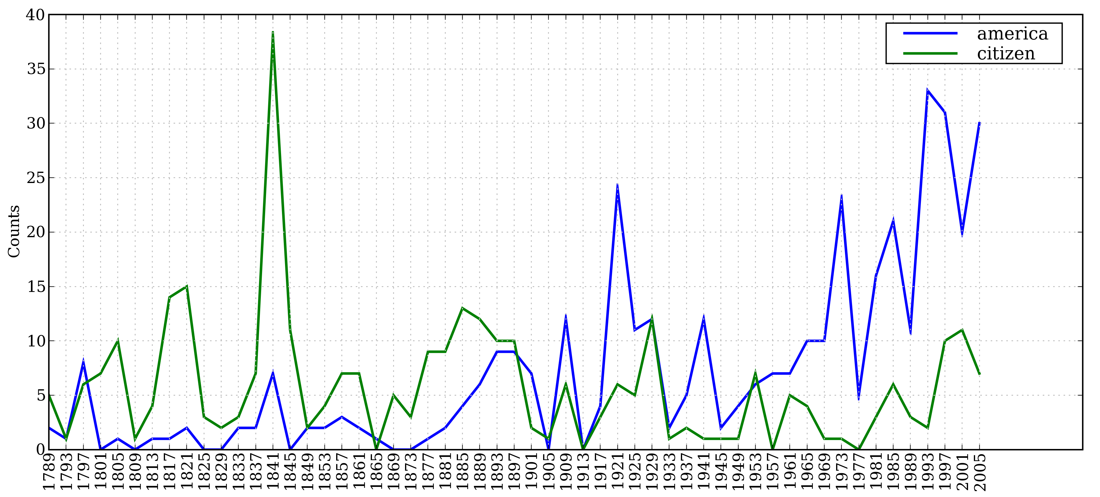
Figure 1.1: Plot of a Conditional Frequency Distribution: all words in the Inaugural Address Corpus that begin with america or citizen are counted; separate counts are kept for each address; these are plotted so that trends in usage over time can be observed; counts are not normalized for document length.
1.6 Annotated Text Corpora
Many text corpora contain linguistic annotations, representing POS tags, named entities, syntactic structures, semantic roles, and so forth. NLTK provides convenient ways to access several of these corpora, and has data packages containing corpora and corpus samples, freely downloadable for use in teaching and research. 1.2 lists some of the corpora. For information about downloading them, see http://nltk.org/data. For more examples of how to access NLTK corpora, please consult the Corpus HOWTO at http://nltk.org/howto.
| Corpus | Compiler | Contents |
|---|---|---|
| Brown Corpus | Francis, Kucera | 15 genres, 1.15M words, tagged, categorized |
| CESS Treebanks | CLiC-UB | 1M words, tagged and parsed (Catalan, Spanish) |
| Chat-80 Data Files | Pereira & Warren | World Geographic Database |
| CMU Pronouncing Dictionary | CMU | 127k entries |
| CoNLL 2000 Chunking Data | CoNLL | 270k words, tagged and chunked |
| CoNLL 2002 Named Entity | CoNLL | 700k words, pos- and named-entity-tagged (Dutch, Spanish) |
| CoNLL 2007 Dependency Treebanks (sel) | CoNLL | 150k words, dependency parsed (Basque, Catalan) |
| Dependency Treebank | Narad | Dependency parsed version of Penn Treebank sample |
| FrameNet | Fillmore, Baker et al | 10k word senses, 170k manually annotated sentences |
| Floresta Treebank | Diana Santos et al | 9k sentences, tagged and parsed (Portuguese) |
| Gazetteer Lists | Various | Lists of cities and countries |
| Genesis Corpus | Misc web sources | 6 texts, 200k words, 6 languages |
| Gutenberg (selections) | Hart, Newby, et al | 18 texts, 2M words |
| Inaugural Address Corpus | CSpan | US Presidential Inaugural Addresses (1789-present) |
| Indian POS-Tagged Corpus | Kumaran et al | 60k words, tagged (Bangla, Hindi, Marathi, Telugu) |
| MacMorpho Corpus | NILC, USP, Brazil | 1M words, tagged (Brazilian Portuguese) |
| Movie Reviews | Pang, Lee | 2k movie reviews with sentiment polarity classification |
| Names Corpus | Kantrowitz, Ross | 8k male and female names |
| NIST 1999 Info Extr (selections) | Garofolo | 63k words, newswire and named-entity SGML markup |
| Nombank | Meyers | 115k propositions, 1400 noun frames |
| NPS Chat Corpus | Forsyth, Martell | 10k IM chat posts, POS-tagged and dialogue-act tagged |
| Open Multilingual WordNet | Bond et al | 15 languages, aligned to English WordNet |
| PP Attachment Corpus | Ratnaparkhi | 28k prepositional phrases, tagged as noun or verb modifiers |
| Proposition Bank | Palmer | 113k propositions, 3300 verb frames |
| Question Classification | Li, Roth | 6k questions, categorized |
| Reuters Corpus | Reuters | 1.3M words, 10k news documents, categorized |
| Roget's Thesaurus | Project Gutenberg | 200k words, formatted text |
| RTE Textual Entailment | Dagan et al | 8k sentence pairs, categorized |
| SEMCOR | Rus, Mihalcea | 880k words, part-of-speech and sense tagged |
| Senseval 2 Corpus | Pedersen | 600k words, part-of-speech and sense tagged |
| SentiWordNet | Esuli, Sebastiani | sentiment scores for 145k WordNet synonym sets |
| Shakespeare texts (selections) | Bosak | 8 books in XML format |
| State of the Union Corpus | CSPAN | 485k words, formatted text |
| Stopwords Corpus | Porter et al | 2,400 stopwords for 11 languages |
| Swadesh Corpus | Wiktionary | comparative wordlists in 24 languages |
| Switchboard Corpus (selections) | LDC | 36 phonecalls, transcribed, parsed |
| Univ Decl of Human Rights | United Nations | 480k words, 300+ languages |
| Penn Treebank (selections) | LDC | 40k words, tagged and parsed |
| TIMIT Corpus (selections) | NIST/LDC | audio files and transcripts for 16 speakers |
| VerbNet 2.1 | Palmer et al | 5k verbs, hierarchically organized, linked to WordNet |
| Wordlist Corpus | OpenOffice.org et al | 960k words and 20k affixes for 8 languages |
| WordNet 3.0 (English) | Miller, Fellbaum | 145k synonym sets |
1.7 Corpora in Other Languages
NLTK comes with corpora for many languages, though in some cases you will need to learn how to manipulate character encodings in Python before using these corpora (see 3.3).
|
The last of these corpora, udhr, contains the Universal Declaration of Human Rights in over 300 languages. The fileids for this corpus include information about the character encoding used in the file, such as UTF8 or Latin1. Let's use a conditional frequency distribution to examine the differences in word lengths for a selection of languages included in the udhr corpus. The output is shown in 1.2 (run the program yourself to see a color plot). Note that True and False are Python's built-in boolean values.
|
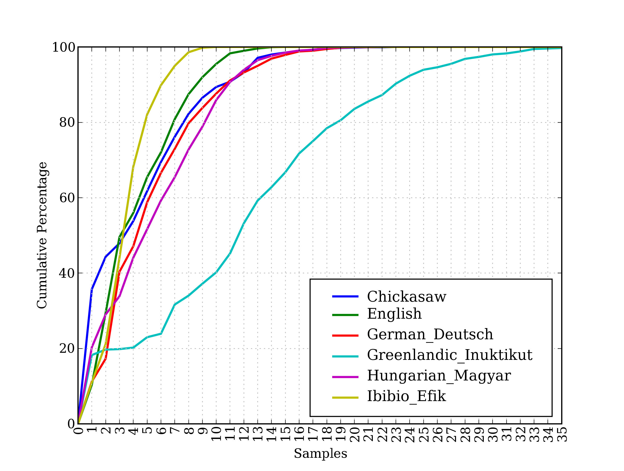
Figure 1.2: Cumulative Word Length Distributions: Six translations of the Universal Declaration of Human Rights are processed; this graph shows that words having 5 or fewer letters account for about 80% of Ibibio text, 60% of German text, and 25% of Inuktitut text.
Note
Your Turn: Pick a language of interest in udhr.fileids(), and define a variable raw_text = udhr.raw(Language-Latin1). Now plot a frequency distribution of the letters of the text using nltk.FreqDist(raw_text).plot().
Unfortunately, for many languages, substantial corpora are not yet available. Often there is insufficient government or industrial support for developing language resources, and individual efforts are piecemeal and hard to discover or re-use. Some languages have no established writing system, or are endangered. (See 7 for suggestions on how to locate language resources.)
1.8 Text Corpus Structure
We have seen a variety of corpus structures so far; these are summarized in 1.3. The simplest kind lacks any structure: it is just a collection of texts. Often, texts are grouped into categories that might correspond to genre, source, author, language, etc. Sometimes these categories overlap, notably in the case of topical categories as a text can be relevant to more than one topic. Occasionally, text collections have temporal structure, news collections being the most common example.
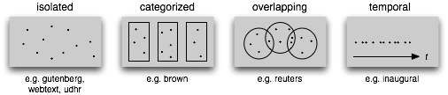
Figure 1.3: Common Structures for Text Corpora: The simplest kind of corpus is a collection of isolated texts with no particular organization; some corpora are structured into categories like genre (Brown Corpus); some categorizations overlap, such as topic categories (Reuters Corpus); other corpora represent language use over time (Inaugural Address Corpus).
| Example | Description |
|---|---|
| fileids() | the files of the corpus |
| fileids([categories]) | the files of the corpus corresponding to these categories |
| categories() | the categories of the corpus |
| categories([fileids]) | the categories of the corpus corresponding to these files |
| raw() | the raw content of the corpus |
| raw(fileids=[f1,f2,f3]) | the raw content of the specified files |
| raw(categories=[c1,c2]) | the raw content of the specified categories |
| words() | the words of the whole corpus |
| words(fileids=[f1,f2,f3]) | the words of the specified fileids |
| words(categories=[c1,c2]) | the words of the specified categories |
| sents() | the sentences of the whole corpus |
| sents(fileids=[f1,f2,f3]) | the sentences of the specified fileids |
| sents(categories=[c1,c2]) | the sentences of the specified categories |
| abspath(fileid) | the location of the given file on disk |
| encoding(fileid) | the encoding of the file (if known) |
| open(fileid) | open a stream for reading the given corpus file |
| root | if the path to the root of locally installed corpus |
| readme() | the contents of the README file of the corpus |
NLTK's corpus readers support efficient access to a variety of corpora, and can be used to work with new corpora. 1.3 lists functionality provided by the corpus readers. We illustrate the difference between some of the corpus access methods below:
|
1.9 Loading your own Corpus
If you have your own collection of text files that you would like to access using
the above methods, you can easily load them with the help of NLTK's
PlaintextCorpusReader. Check the location of your files on your file system; in
the following example, we have taken this to be the directory
/usr/share/dict. Whatever the location, set this to be the value of
corpus_root .
The second parameter of the PlaintextCorpusReader initializer ![[2]](callouts/callout2.gif) can be a list of fileids, like ['a.txt', 'test/b.txt'],
or a pattern that matches all fileids, like '[abc]/.*\.txt'
(see 3.4 for information
about regular expressions).
can be a list of fileids, like ['a.txt', 'test/b.txt'],
or a pattern that matches all fileids, like '[abc]/.*\.txt'
(see 3.4 for information
about regular expressions).
|
As another example, suppose you have your own local copy of Penn Treebank (release 3),
in C:\corpora. We can use the BracketParseCorpusReader to access this
corpus. We specify the corpus_root to be the location of the parsed Wall Street
Journal component of the corpus , and give a file_pattern
that matches the files contained within its subfolders (using forward slashes).
|
2 Conditional Frequency Distributions
We introduced frequency distributions in 3. We saw that given some list mylist of words or other items, FreqDist(mylist) would compute the number of occurrences of each item in the list. Here we will generalize this idea.
When the texts of a corpus are divided into several categories, by genre, topic, author, etc, we can maintain separate frequency distributions for each category. This will allow us to study systematic differences between the categories. In the previous section we achieved this using NLTK's ConditionalFreqDist data type. A conditional frequency distribution is a collection of frequency distributions, each one for a different "condition". The condition will often be the category of the text. 2.1 depicts a fragment of a conditional frequency distribution having just two conditions, one for news text and one for romance text.
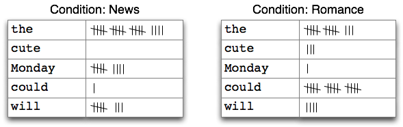
Figure 2.1: Counting Words Appearing in a Text Collection (a conditional frequency distribution)
2.1 Conditions and Events
A frequency distribution counts observable events,
such as the appearance of words in a text. A conditional
frequency distribution needs to pair each event with a condition.
So instead of processing a sequence of words ,
we have to process a sequence of pairs :
|
Each pair has the form (condition, event). If we were processing the entire Brown Corpus by genre there would be 15 conditions (one per genre), and 1,161,192 events (one per word).
2.2 Counting Words by Genre
In 1 we saw a conditional frequency distribution where the condition was the section of the Brown Corpus, and for each condition we counted words. Whereas FreqDist() takes a simple list as input, ConditionalFreqDist() takes a list of pairs.
|
Let's break this down, and look at just two genres, news and romance.
For each genre , we loop over every word in the genre ![[3]](callouts/callout3.gif) ,
producing pairs consisting of the genre and the word :
,
producing pairs consisting of the genre and the word :
|
So, as we can see below,
pairs at the beginning of the list genre_word will be of the form
('news', word) , while those at the end will be of the form
('romance', word) .
|
We can now use this list of pairs to create a ConditionalFreqDist, and
save it in a variable cfd. As usual, we can type the name of the
variable to inspect it , and verify it has two conditions :
|
Let's access the two conditions, and satisfy ourselves that each is just a frequency distribution:
|
2.3 Plotting and Tabulating Distributions
Apart from combining two or more frequency distributions, and being easy to initialize, a ConditionalFreqDist provides some useful methods for tabulation and plotting.
The plot in 1.1 was based on a conditional frequency distribution
reproduced in the code below.
The condition is either of the words america or citizen ,
and the counts being plotted are the number of times the word occured in a particular speech.
It exploits the fact that the filename for each speech, e.g., 1865-Lincoln.txt
contains the year as the first four characters .
This code generates the pair ('america', '1865') for
every instance of a word whose lowercased form starts with america
— such as Americans — in the file 1865-Lincoln.txt.
|
The plot in 1.2 was also based on a conditional frequency distribution,
reproduced below. This time, the condition is the name of the language
and the counts being plotted are derived from word lengths .
It exploits the fact that the filename for each language is the language name followed
by '-Latin1' (the character encoding).
|
In the plot() and tabulate() methods, we can optionally specify which conditions to display with a conditions= parameter. When we omit it, we get all the conditions. Similarly, we can limit the samples to display with a samples= parameter. This makes it possible to load a large quantity of data into a conditional frequency distribution, and then to explore it by plotting or tabulating selected conditions and samples. It also gives us full control over the order of conditions and samples in any displays. For example, we can tabulate the cumulative frequency data just for two languages, and for words less than 10 characters long, as shown below. We interpret the last cell on the top row to mean that 1,638 words of the English text have 9 or fewer letters.
|
Note
Your Turn: Working with the news and romance genres from the Brown Corpus, find out which days of the week are most newsworthy, and which are most romantic. Define a variable called days containing a list of days of the week, i.e. ['Monday', ...]. Now tabulate the counts for these words using cfd.tabulate(samples=days). Now try the same thing using plot in place of tabulate. You may control the output order of days with the help of an extra parameter: samples=['Monday', ...].
You may have noticed that the multi-line expressions we have been using with conditional frequency distributions look like list comprehensions, but without the brackets. In general, when we use a list comprehension as a parameter to a function, like set([w.lower() for w in t]), we are permitted to omit the square brackets and just write: set(w.lower() for w in t). (See the discussion of "generator expressions" in 4.2 for more about this.)
2.4 Generating Random Text with Bigrams
We can use a conditional frequency distribution to create a table of bigrams (word pairs). (We introducted bigrams in 3.) The bigrams() function takes a list of words and builds a list of consecutive word pairs. Remember that, in order to see the result and not a cryptic "generator object", we need to use the list() function:
|
In 2.2, we treat each word as a condition, and for each one we effectively create a frequency distribution over the following words. The function generate_model() contains a simple loop to generate text. When we call the function, we choose a word (such as 'living') as our initial context, then once inside the loop, we print the current value of the variable word, and reset word to be the most likely token in that context (using max()); next time through the loop, we use that word as our new context. As you can see by inspecting the output, this simple approach to text generation tends to get stuck in loops; another method would be to randomly choose the next word from among the available words.
| ||
| ||
Example 2.2 (code_random_text.py): Figure 2.2: Generating Random Text: this program obtains all bigrams from the text of the book of Genesis, then constructs a conditional frequency distribution to record which words are most likely to follow a given word; e.g., after the word living, the most likely word is creature; the generate_model() function uses this data, and a seed word, to generate random text. |
Conditional frequency distributions are a useful data structure for many NLP tasks. Their commonly-used methods are summarized in 2.1.
| Example | Description |
|---|---|
| cfdist = ConditionalFreqDist(pairs) | create a conditional frequency distribution from a list of pairs |
| cfdist.conditions() | the conditions |
| cfdist[condition] | the frequency distribution for this condition |
| cfdist[condition][sample] | frequency for the given sample for this condition |
| cfdist.tabulate() | tabulate the conditional frequency distribution |
| cfdist.tabulate(samples, conditions) | tabulation limited to the specified samples and conditions |
| cfdist.plot() | graphical plot of the conditional frequency distribution |
| cfdist.plot(samples, conditions) | graphical plot limited to the specified samples and conditions |
| cfdist1 < cfdist2 | test if samples in cfdist1 occur less frequently than in cfdist2 |
3 More Python: Reusing Code
By this time you've probably typed and retyped a lot of code in the Python interactive interpreter. If you mess up when retyping a complex example you have to enter it again. Using the arrow keys to access and modify previous commands is helpful but only goes so far. In this section we see two important ways to reuse code: text editors and Python functions.
3.1 Creating Programs with a Text Editor
The Python interactive interpreter performs your instructions as soon as you type them. Often, it is better to compose a multi-line program using a text editor, then ask Python to run the whole program at once. Using IDLE, you can do this by going to the File menu and opening a new window. Try this now, and enter the following one-line program:
print('Monty Python')
Save this program in a file called monty.py, then go to the Run menu, and select the command Run Module. (We'll learn what modules are shortly.) The result in the main IDLE window should look like this:
|
You can also type from monty import * and it will do the same thing.
From now on, you have a choice of using the interactive interpreter or a text editor to create your programs. It is often convenient to test your ideas using the interpreter, revising a line of code until it does what you expect. Once you're ready, you can paste the code (minus any >>> or ... prompts) into the text editor, continue to expand it, and finally save the program in a file so that you don't have to type it in again later. Give the file a short but descriptive name, using all lowercase letters and separating words with underscore, and using the .py filename extension, e.g., monty_python.py.
Note
Important: Our inline code examples include the >>> and ... prompts as if we are interacting directly with the interpreter. As they get more complicated, you should instead type them into the editor, without the prompts, and run them from the editor as shown above. When we provide longer programs in this book, we will leave out the prompts to remind you to type them into a file rather than using the interpreter. You can see this already in 2.2 above. Note that it still includes a couple of lines with the Python prompt; this is the interactive part of the task where you inspect some data and invoke a function. Remember that all code samples like 2.2 are downloadable from http://nltk.org/.
3.2 Functions
Suppose that you work on analyzing text that involves different forms of the same word, and that part of your program needs to work out the plural form of a given singular noun. Suppose it needs to do this work in two places, once when it is processing some texts, and again when it is processing user input.
Rather than repeating the same code several times over, it is more efficient and reliable to localize this work inside a function. A function is just a named block of code that performs some well-defined task, as we saw in 1. A function is usually defined to take some inputs, using special variables known as parameters, and it may produce a result, also known as a return value. We define a function using the keyword def followed by the function name and any input parameters, followed by the body of the function. Here's the function we saw in 1 (including the import statement that is needed for Python 2, in order to make division behave as expected):
|
We use the keyword return to indicate the value that is produced as output by the function. In the above example, all the work of the function is done in the return statement. Here's an equivalent definition which does the same work using multiple lines of code. We'll change the parameter name from text to my_text_data to remind you that this is an arbitrary choice:
|
Notice that we've created some new variables inside the body of the function. These are local variables and are not accessible outside the function. So now we have defined a function with the name lexical_diversity. But just defining it won't produce any output! Functions do nothing until they are "called" (or "invoked"):
|
Let's return to our earlier scenario, and actually define a simple function to work out English plurals. The function plural() in 3.1 takes a singular noun and generates a plural form, though it is not always correct. (We'll discuss functions at greater length in 4.4.)
| ||
| ||
Example 3.1 (code_plural.py): Figure 3.1: A Python Function: this function tries to work out the plural form of any English noun; the keyword def (define) is followed by the function name, then a parameter inside parentheses, and a colon; the body of the function is the indented block of code; it tries to recognize patterns within the word and process the word accordingly; e.g., if the word ends with y, delete the y and add ies. |
The endswith() function is always associated with a string object (e.g., word in 3.1). To call such functions, we give the name of the object, a period, and then the name of the function. These functions are usually known as methods.
3.3 Modules
Over time you will find that you create a variety of useful little text processing functions, and you end up copying them from old programs to new ones. Which file contains the latest version of the function you want to use? It makes life a lot easier if you can collect your work into a single place, and access previously defined functions without making copies.
To do this, save your function(s) in a file called (say) text_proc.py. Now, you can access your work simply by importing it from the file:
|
Our plural function obviously has an error, since the plural of fan is fans. Instead of typing in a new version of the function, we can simply edit the existing one. Thus, at every stage, there is only one version of our plural function, and no confusion about which one is being used.
A collection of variable and function definitions in a file is called a Python module. A collection of related modules is called a package. NLTK's code for processing the Brown Corpus is an example of a module, and its collection of code for processing all the different corpora is an example of a package. NLTK itself is a set of packages, sometimes called a library.
Caution!
If you are creating a file to contain some of your Python code, do not name your file nltk.py: it may get imported in place of the "real" NLTK package. When it imports modules, Python first looks in the current directory (folder).
4 Lexical Resources
A lexicon, or lexical resource, is a collection of words and/or phrases along with associated information such as part of speech and sense definitions. Lexical resources are secondary to texts, and are usually created and enriched with the help of texts. For example, if we have defined a text my_text, then vocab = sorted(set(my_text)) builds the vocabulary of my_text, while word_freq = FreqDist(my_text) counts the frequency of each word in the text. Both of vocab and word_freq are simple lexical resources. Similarly, a concordance like the one we saw in 1 gives us information about word usage that might help in the preparation of a dictionary. Standard terminology for lexicons is illustrated in 4.1. A lexical entry consists of a headword (also known as a lemma) along with additional information such as the part of speech and the sense definition. Two distinct words having the same spelling are called homonyms.
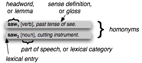
Figure 4.1: Lexicon Terminology: lexical entries for two lemmas having the same spelling (homonyms), providing part of speech and gloss information.
The simplest kind of lexicon is nothing more than a sorted list of words. Sophisticated lexicons include complex structure within and across the individual entries. In this section we'll look at some lexical resources included with NLTK.
4.1 Wordlist Corpora
NLTK includes some corpora that are nothing more than wordlists. The Words Corpus is the /usr/share/dict/words file from Unix, used by some spell checkers. We can use it to find unusual or mis-spelt words in a text corpus, as shown in 4.2.
| ||
Example 4.2 (code_unusual.py): Figure 4.2: Filtering a Text: this program computes the vocabulary of a text, then removes all items that occur in an existing wordlist, leaving just the uncommon or mis-spelt words. |
There is also a corpus of stopwords, that is, high-frequency words like the, to and also that we sometimes want to filter out of a document before further processing. Stopwords usually have little lexical content, and their presence in a text fails to distinguish it from other texts.
|
Let's define a function to compute what fraction of words in a text are not in the stopwords list:
|
Thus, with the help of stopwords we filter out over a quarter of the words of the text. Notice that we've combined two different kinds of corpus here, using a lexical resource to filter the content of a text corpus.
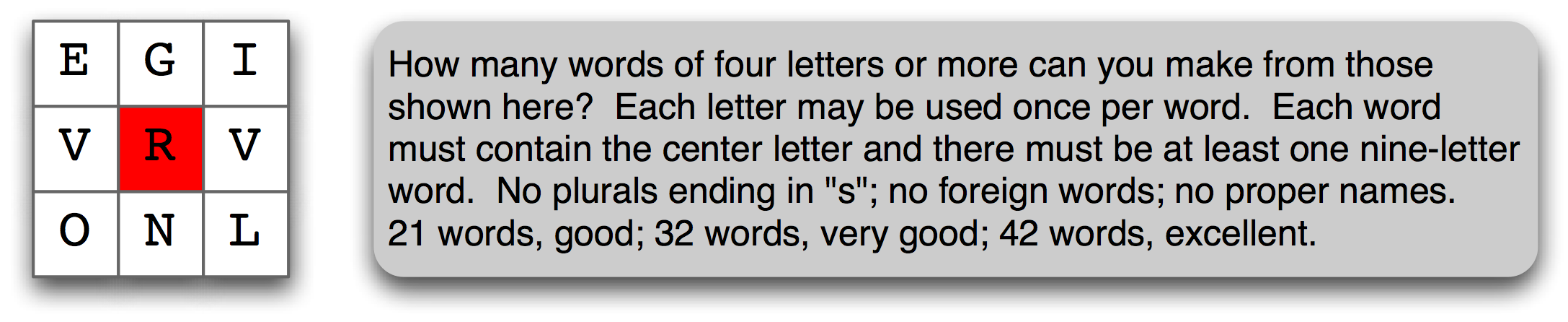
Figure 4.3: A Word Puzzle: a grid of randomly chosen letters with rules for creating words out of the letters; this puzzle is known as "Target."
A wordlist is useful for solving word puzzles, such as the one in 4.3.
Our program iterates through every word and, for each one, checks whether it meets
the conditions. It is easy to check obligatory letter
and length constraints (and we'll
only look for words with six or more letters here).
It is trickier to check that candidate solutions only use combinations of the
supplied letters, especially since some of the supplied letters
appear twice (here, the letter v).
The FreqDist comparison method permits us to check that
the frequency of each letter in the candidate word is less than or equal
to the frequency of the corresponding letter in the puzzle.
|
One more wordlist corpus is the Names corpus, containing 8,000 first names categorized by gender. The male and female names are stored in separate files. Let's find names which appear in both files, i.e. names that are ambiguous for gender:
|
It is well known that names ending in the letter a are almost always female. We can see this and some other patterns in the graph in 4.4, produced by the following code. Remember that name[-1] is the last letter of name.
|
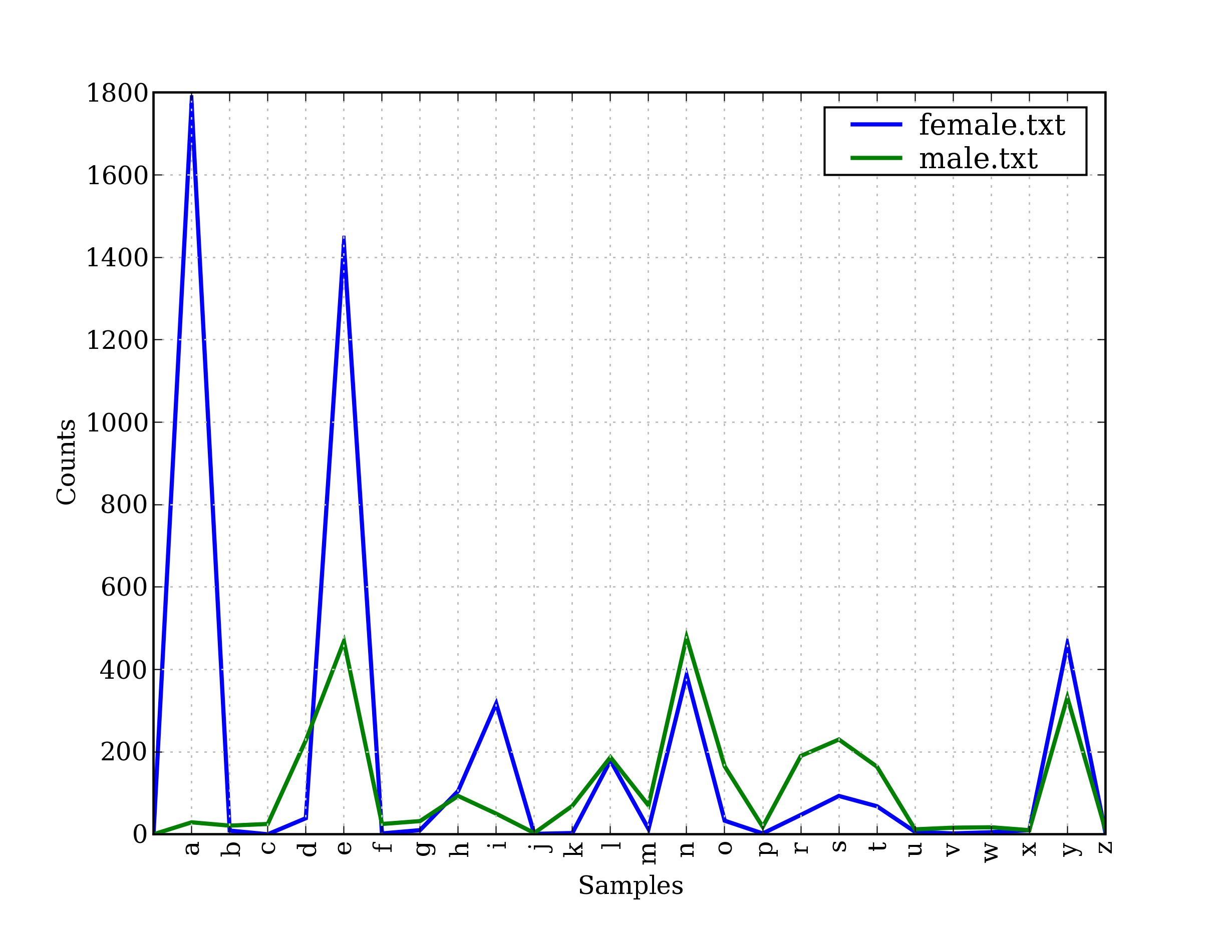
Figure 4.4: Conditional Frequency Distribution: this plot shows the number of female and male names ending with each letter of the alphabet; most names ending with a, e or i are female; names ending in h and l are equally likely to be male or female; names ending in k, o, r, s, and t are likely to be male.
4.2 A Pronouncing Dictionary
A slightly richer kind of lexical resource is a table (or spreadsheet), containing a word plus some properties in each row. NLTK includes the CMU Pronouncing Dictionary for US English, which was designed for use by speech synthesizers.
|
For each word, this lexicon provides a list of phonetic codes — distinct labels for each contrastive sound — known as phones. Observe that fire has two pronunciations (in US English): the one-syllable F AY1 R, and the two-syllable F AY1 ER0. The symbols in the CMU Pronouncing Dictionary are from the Arpabet, described in more detail at http://en.wikipedia.org/wiki/Arpabet
Each entry consists of two parts, and we can
process these individually using a more complex version of the for statement.
Instead of writing for entry in entries:, we replace
entry with two variable names, word, pron .
Now, each time through the loop, word is assigned the first part of the
entry, and pron is assigned the second part of the entry:
|
The above program scans the lexicon looking for entries whose pronunciation consists of
three phones . If the condition is true, it assigns the contents
of pron to three new variables ph1, ph2 and ph3. Notice the unusual
form of the statement which does that work .
Here's another example of the same for statement, this time used inside a list comprehension. This program finds all words whose pronunciation ends with a syllable sounding like nicks. You could use this method to find rhyming words.
|
Notice that the one pronunciation is spelt in several ways: nics, niks, nix, even ntic's with a silent t, for the word atlantic's. Let's look for some other mismatches between pronunciation and writing. Can you summarize the purpose of the following examples and explain how they work?
|
The phones contain digits to represent primary stress (1), secondary stress (2) and no stress (0). As our final example, we define a function to extract the stress digits and then scan our lexicon to find words having a particular stress pattern.
|
Note
A subtlety of the above program is that our user-defined function stress() is invoked inside the condition of a list comprehension. There is also a doubly-nested for loop. There's a lot going on here and you might want to return to this once you've had more experience using list comprehensions.
We can use a conditional frequency distribution to help us find minimally-contrasting
sets of words. Here we find all the p-words consisting of three sounds ,
and group them according to their first and last sounds .
|
Rather than iterating over the whole dictionary, we can also access it
by looking up particular words. We will use Python's dictionary data
structure, which we will study systematically in 3.
We look up a dictionary by giving its name followed by a key
(such as the word 'fire') inside square brackets .
|
If we try to look up a non-existent key , we get a KeyError.
This is similar to what happens when we index a list with an
integer that is too large, producing an IndexError.
The word blog is missing from the pronouncing dictionary,
so we tweak our version by assigning a value for this key
(this has no effect on the NLTK corpus; next time we access it,
blog will still be absent).
We can use any lexical resource to process a text, e.g., to filter out words having some lexical property (like nouns), or mapping every word of the text. For example, the following text-to-speech function looks up each word of the text in the pronunciation dictionary.
|
4.3 Comparative Wordlists
Another example of a tabular lexicon is the comparative wordlist. NLTK includes so-called Swadesh wordlists, lists of about 200 common words in several languages. The languages are identified using an ISO 639 two-letter code.
|
We can access cognate words from multiple languages using the entries() method, specifying a list of languages. With one further step we can convert this into a simple dictionary (we'll learn about dict() in 3).
|
We can make our simple translator more useful by adding other source languages. Let's get the German-English and Spanish-English pairs, convert each to a dictionary using dict(), then update our original translate dictionary with these additional mappings:
|
We can compare words in various Germanic and Romance languages:
|
4.4 Shoebox and Toolbox Lexicons
Perhaps the single most popular tool used by linguists for managing data is Toolbox, previously known as Shoebox since it replaces the field linguist's traditional shoebox full of file cards. Toolbox is freely downloadable from http://www.sil.org/computing/toolbox/.
A Toolbox file consists of a collection of entries, where each entry is made up of one or more fields. Most fields are optional or repeatable, which means that this kind of lexical resource cannot be treated as a table or spreadsheet.
Here is a dictionary for the Rotokas language. We see just the first entry, for the word kaa meaning "to gag":
|
Entries consist of a series of attribute-value pairs, like ('ps', 'V') to indicate that the part-of-speech is 'V' (verb), and ('ge', 'gag') to indicate that the gloss-into-English is 'gag'. The last three pairs contain an example sentence in Rotokas and its translations into Tok Pisin and English.
The loose structure of Toolbox files makes it hard for us to do much more with them at this stage. XML provides a powerful way to process this kind of corpus and we will return to this topic in 11..
Note
The Rotokas language is spoken on the island of Bougainville, Papua New Guinea. This lexicon was contributed to NLTK by Stuart Robinson. Rotokas is notable for having an inventory of just 12 phonemes (contrastive sounds), http://en.wikipedia.org/wiki/Rotokas_language
5 WordNet
WordNet is a semantically-oriented dictionary of English, similar to a traditional thesaurus but with a richer structure. NLTK includes the English WordNet, with 155,287 words and 117,659 synonym sets. We'll begin by looking at synonyms and how they are accessed in WordNet.
5.1 Senses and Synonyms
Consider the sentence in (1a). If we replace the word motorcar in (1a) by automobile, to get (1b), the meaning of the sentence stays pretty much the same:
| (1) |
|
Since everything else in the sentence has remained unchanged, we can conclude that the words motorcar and automobile have the same meaning, i.e. they are synonyms. We can explore these words with the help of WordNet:
|
Thus, motorcar has just one possible meaning and it is identified as car.n.01, the first noun sense of car. The entity car.n.01 is called a synset, or "synonym set", a collection of synonymous words (or "lemmas"):
|
Each word of a synset can have several meanings, e.g., car can also signify a train carriage, a gondola, or an elevator car. However, we are only interested in the single meaning that is common to all words of the above synset. Synsets also come with a prose definition and some example sentences:
|
Although definitions help humans to understand the intended meaning of a synset,
the words of the synset are often more useful for our programs.
To eliminate ambiguity, we will identify these words as
car.n.01.automobile, car.n.01.motorcar, and so on.
This pairing of a synset with a word is called a lemma.
We can get all the lemmas for a given synset ,
look up a particular lemma ,
get the synset corresponding to a lemma ,
and get the "name" of a lemma ![[4]](callouts/callout4.gif) :
:
|
Unlike the word motorcar, which is unambiguous and has one synset, the word car is ambiguous, having five synsets:
|
For convenience, we can access all the lemmas involving the word car as follows.
|
Note
Your Turn: Write down all the senses of the word dish that you can think of. Now, explore this word with the help of WordNet, using the same operations we used above.
5.2 The WordNet Hierarchy
WordNet synsets correspond to abstract concepts, and they don't always have corresponding words in English. These concepts are linked together in a hierarchy. Some concepts are very general, such as Entity, State, Event — these are called unique beginners or root synsets. Others, such as gas guzzler and hatchback, are much more specific. A small portion of a concept hierarchy is illustrated in 5.1.
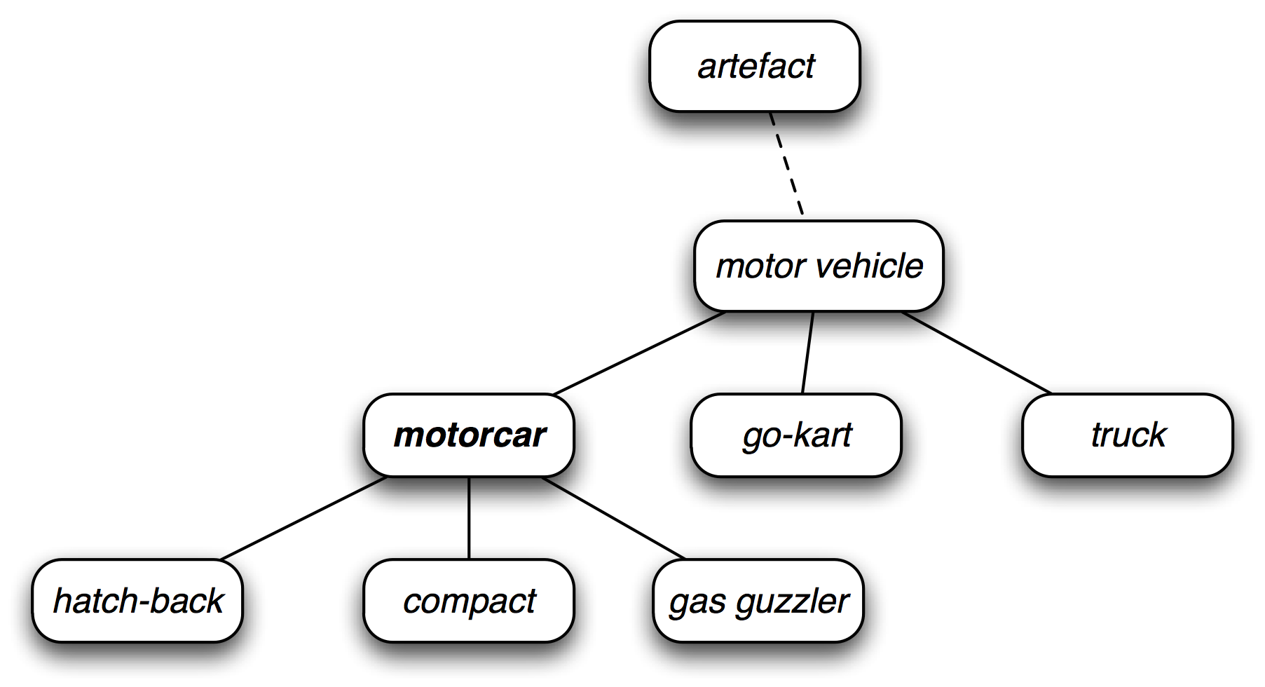
Figure 5.1: Fragment of WordNet Concept Hierarchy: nodes correspond to synsets; edges indicate the hypernym/hyponym relation, i.e. the relation between superordinate and subordinate concepts.
WordNet makes it easy to navigate between concepts. For example, given a concept like motorcar, we can look at the concepts that are more specific; the (immediate) hyponyms.
|
We can also navigate up the hierarchy by visiting hypernyms. Some words have multiple paths, because they can be classified in more than one way. There are two paths between car.n.01 and entity.n.01 because wheeled_vehicle.n.01 can be classified as both a vehicle and a container.
|
We can get the most general hypernyms (or root hypernyms) of a synset as follows:
|
Note
Your Turn: Try out NLTK's convenient graphical WordNet browser: nltk.app.wordnet(). Explore the WordNet hierarchy by following the hypernym and hyponym links.
5.3 More Lexical Relations
Hypernyms and hyponyms are called lexical relations because they relate one synset to another. These two relations navigate up and down the "is-a" hierarchy. Another important way to navigate the WordNet network is from items to their components (meronyms) or to the things they are contained in (holonyms). For example, the parts of a tree are its trunk, crown, and so on; the part_meronyms(). The substance a tree is made of includes heartwood and sapwood; the substance_meronyms(). A collection of trees forms a forest; the member_holonyms():
|
To see just how intricate things can get, consider the word mint, which has several closely-related senses. We can see that mint.n.04 is part of mint.n.02 and the substance from which mint.n.05 is made.
|
There are also relationships between verbs. For example, the act of walking involves the act of stepping, so walking entails stepping. Some verbs have multiple entailments:
|
Some lexical relationships hold between lemmas, e.g., antonymy:
|
You can see the lexical relations, and the other methods defined on a synset, using dir(), for example: dir(wn.synset('harmony.n.02')).
5.4 Semantic Similarity
We have seen that synsets are linked by a complex network of lexical relations. Given a particular synset, we can traverse the WordNet network to find synsets with related meanings. Knowing which words are semantically related is useful for indexing a collection of texts, so that a search for a general term like vehicle will match documents containing specific terms like limousine.
Recall that each synset has one or more hypernym paths that link it to a root hypernym such as entity.n.01. Two synsets linked to the same root may have several hypernyms in common (cf 5.1). If two synsets share a very specific hypernym — one that is low down in the hypernym hierarchy — they must be closely related.
|
Of course we know that whale is very specific (and baleen whale even more so), while vertebrate is more general and entity is completely general. We can quantify this concept of generality by looking up the depth of each synset:
|
Similarity measures have been defined over the collection of WordNet synsets which incorporate the above insight. For example, path_similarity assigns a score in the range 0–1 based on the shortest path that connects the concepts in the hypernym hierarchy (-1 is returned in those cases where a path cannot be found). Comparing a synset with itself will return 1. Consider the following similarity scores, relating right whale to minke whale, orca, tortoise, and novel. Although the numbers won't mean much, they decrease as we move away from the semantic space of sea creatures to inanimate objects.
|
Note
Several other similarity measures are available; you can type help(wn) for more information. NLTK also includes VerbNet, a hierarhical verb lexicon linked to WordNet. It can be accessed with nltk.corpus.verbnet.
6 Summary
- A text corpus is a large, structured collection of texts. NLTK comes with many corpora, e.g., the Brown Corpus, nltk.corpus.brown.
- Some text corpora are categorized, e.g., by genre or topic; sometimes the categories of a corpus overlap each other.
- A conditional frequency distribution is a collection of frequency distributions, each one for a different condition. They can be used for counting word frequencies, given a context or a genre.
- Python programs more than a few lines long should be entered using a text editor, saved to a file with a .py extension, and accessed using an import statement.
- Python functions permit you to associate a name with a particular block of code, and re-use that code as often as necessary.
- Some functions, known as "methods", are associated with an object and we give the object name followed by a period followed by the function, like this: x.funct(y), e.g., word.isalpha().
- To find out about some variable v, type help(v) in the Python interactive interpreter to read the help entry for this kind of object.
- WordNet is a semantically-oriented dictionary of English, consisting of synonym sets — or synsets — and organized into a network.
- Some functions are not available by default, but must be accessed using Python's import statement.
7 Further Reading
Extra materials for this chapter are posted at http://nltk.org/, including links to freely available resources on the web. The corpus methods are summarized in the Corpus HOWTO, at http://nltk.org/howto, and documented extensively in the online API documentation.
Significant sources of published corpora are the Linguistic Data Consortium (LDC) and the European Language Resources Agency (ELRA). Hundreds of annotated text and speech corpora are available in dozens of languages. Non-commercial licences permit the data to be used in teaching and research. For some corpora, commercial licenses are also available (but for a higher fee).
A good tool for creating annotated text corpora is called Brat, and available from http://brat.nlplab.org/.
These and many other language resources have been documented using OLAC Metadata, and can be searched via the OLAC homepage at http://www.language-archives.org/. Corpora List is a mailing list for discussions about corpora, and you can find resources by searching the list archives or posting to the list. The most complete inventory of the world's languages is Ethnologue, http://www.ethnologue.com/. Of 7,000 languages, only a few dozen have substantial digital resources suitable for use in NLP.
This chapter has touched on the field of Corpus Linguistics. Other useful books in this area include (Biber, Conrad, & Reppen, 1998), (McEnery, 2006), (Meyer, 2002), (Sampson & McCarthy, 2005), (Scott & Tribble, 2006). Further readings in quantitative data analysis in linguistics are: (Baayen, 2008), (Gries, 2009), (Woods, Fletcher, & Hughes, 1986).
The original description of WordNet is (Fellbaum, 1998). Although WordNet was originally developed for research in psycholinguistics, it is now widely used in NLP and Information Retrieval. WordNets are being developed for many other languages, as documented at http://www.globalwordnet.org/. For a study of WordNet similarity measures, see (Budanitsky & Hirst, 2006).
Other topics touched on in this chapter were phonetics and lexical semantics, and we refer readers to chapters 7 and 20 of (Jurafsky & Martin, 2008).
8 Exercises
- ☼ Create a variable phrase containing a list of words. Review the operations described in the previous chapter, including addition, multiplication, indexing, slicing, and sorting.
- ☼ Use the corpus module to explore austen-persuasion.txt. How many word tokens does this book have? How many word types?
- ☼ Use the Brown corpus reader nltk.corpus.brown.words() or the Web text corpus reader nltk.corpus.webtext.words() to access some sample text in two different genres.
- ☼ Read in the texts of the State of the Union addresses, using the state_union corpus reader. Count occurrences of men, women, and people in each document. What has happened to the usage of these words over time?
- ☼ Investigate the holonym-meronym relations for some nouns. Remember that there are three kinds of holonym-meronym relation, so you need to use: member_meronyms(), part_meronyms(), substance_meronyms(), member_holonyms(), part_holonyms(), and substance_holonyms().
- ☼ In the discussion of comparative wordlists, we created an object called translate which you could look up using words in both German and Spanish in order to get corresponding words in English. What problem might arise with this approach? Can you suggest a way to avoid this problem?
- ☼ According to Strunk and White's Elements of Style, the word however, used at the start of a sentence, means "in whatever way" or "to whatever extent", and not "nevertheless". They give this example of correct usage: However you advise him, he will probably do as he thinks best. (http://www.bartleby.com/141/strunk3.html) Use the concordance tool to study actual usage of this word in the various texts we have been considering. See also the LanguageLog posting "Fossilized prejudices about 'however'" at http://itre.cis.upenn.edu/~myl/languagelog/archives/001913.html
- ◑ Define a conditional frequency distribution over the Names corpus that allows you to see which initial letters are more frequent for males vs. females (cf. 4.4).
- ◑ Pick a pair of texts and study the differences between them, in terms of vocabulary, vocabulary richness, genre, etc. Can you find pairs of words which have quite different meanings across the two texts, such as monstrous in Moby Dick and in Sense and Sensibility?
- ◑ Read the BBC News article: UK's Vicky Pollards 'left behind' http://news.bbc.co.uk/1/hi/education/6173441.stm. The article gives the following statistic about teen language: "the top 20 words used, including yeah, no, but and like, account for around a third of all words." How many word types account for a third of all word tokens, for a variety of text sources? What do you conclude about this statistic? Read more about this on LanguageLog, at http://itre.cis.upenn.edu/~myl/languagelog/archives/003993.html.
- ◑ Investigate the table of modal distributions and look for other patterns. Try to explain them in terms of your own impressionistic understanding of the different genres. Can you find other closed classes of words that exhibit significant differences across different genres?
- ◑ The CMU Pronouncing Dictionary contains multiple pronunciations for certain words. How many distinct words does it contain? What fraction of words in this dictionary have more than one possible pronunciation?
- ◑ What percentage of noun synsets have no hyponyms? You can get all noun synsets using wn.all_synsets('n').
- ◑ Define a function supergloss(s) that takes a synset s as its argument and returns a string consisting of the concatenation of the definition of s, and the definitions of all the hypernyms and hyponyms of s.
- ◑ Write a program to find all words that occur at least three times in the Brown Corpus.
- ◑ Write a program to generate a table of lexical diversity scores (i.e. token/type ratios), as we saw in 1.1. Include the full set of Brown Corpus genres (nltk.corpus.brown.categories()). Which genre has the lowest diversity (greatest number of tokens per type)? Is this what you would have expected?
- ◑ Write a function that finds the 50 most frequently occurring words of a text that are not stopwords.
- ◑ Write a program to print the 50 most frequent bigrams (pairs of adjacent words) of a text, omitting bigrams that contain stopwords.
- ◑ Write a program to create a table of word frequencies by genre, like the one given in 1 for modals. Choose your own words and try to find words whose presence (or absence) is typical of a genre. Discuss your findings.
- ◑ Write a function word_freq() that takes a word and the name of a section of the Brown Corpus as arguments, and computes the frequency of the word in that section of the corpus.
- ◑ Write a program to guess the number of syllables contained in a text, making use of the CMU Pronouncing Dictionary.
- ◑ Define a function hedge(text) which processes a text and produces a new version with the word 'like' between every third word.
- ★ Zipf's Law:
Let f(w) be the frequency of a word w in free text. Suppose that
all the words of a text are ranked according to their frequency,
with the most frequent word first. Zipf's law states that the
frequency of a word type is inversely proportional to its rank
(i.e. f × r = k, for some constant k). For example, the 50th most
common word type should occur three times as frequently as the
150th most common word type.
- Write a function to process a large text and plot word frequency against word rank using pylab.plot. Do you confirm Zipf's law? (Hint: it helps to use a logarithmic scale). What is going on at the extreme ends of the plotted line?
- Generate random text, e.g., using random.choice("abcdefg "), taking care to include the space character. You will need to import random first. Use the string concatenation operator to accumulate characters into a (very) long string. Then tokenize this string, and generate the Zipf plot as before, and compare the two plots. What do you make of Zipf's Law in the light of this?
- ★ Modify the text generation program in 2.2 further, to
do the following tasks:
- Store the n most likely words in a list words then randomly choose a word from the list using random.choice(). (You will need to import random first.)
- Select a particular genre, such as a section of the Brown Corpus, or a genesis translation, one of the Gutenberg texts, or one of the Web texts. Train the model on this corpus and get it to generate random text. You may have to experiment with different start words. How intelligible is the text? Discuss the strengths and weaknesses of this method of generating random text.
- Now train your system using two distinct genres and experiment with generating text in the hybrid genre. Discuss your observations.
- ★ Define a function find_language() that takes a string as its argument, and returns a list of languages that have that string as a word. Use the udhr corpus and limit your searches to files in the Latin-1 encoding.
- ★ What is the branching factor of the noun hypernym hierarchy? I.e. for every noun synset that has hyponyms — or children in the hypernym hierarchy — how many do they have on average? You can get all noun synsets using wn.all_synsets('n').
- ★ The polysemy of a word is the number of senses it has. Using WordNet, we can determine that the noun dog has 7 senses with: len(wn.synsets('dog', 'n')). Compute the average polysemy of nouns, verbs, adjectives and adverbs according to WordNet.
- ★ Use one of the predefined similarity measures to score the similarity of each of the following pairs of words. Rank the pairs in order of decreasing similarity. How close is your ranking to the order given here, an order that was established experimentally by (Miller & Charles, 1998): car-automobile, gem-jewel, journey-voyage, boy-lad, coast-shore, asylum-madhouse, magician-wizard, midday-noon, furnace-stove, food-fruit, bird-cock, bird-crane, tool-implement, brother-monk, lad-brother, crane-implement, journey-car, monk-oracle, cemetery-woodland, food-rooster, coast-hill, forest-graveyard, shore-woodland, monk-slave, coast-forest, lad-wizard, chord-smile, glass-magician, rooster-voyage, noon-string.
About this document...
UPDATED FOR NLTK 3.0. This is a chapter from Natural Language Processing with Python, by Steven Bird, Ewan Klein and Edward Loper, Copyright © 2019 the authors. It is distributed with the Natural Language Toolkit [http://nltk.org/], Version 3.0, under the terms of the Creative Commons Attribution-Noncommercial-No Derivative Works 3.0 United States License [http://creativecommons.org/licenses/by-nc-nd/3.0/us/].
This document was built on Wed 4 Sep 2019 11:40:48 ACST