4 Writing Structured Programs
By now you will have a sense of the capabilities of the Python programming language for processing natural language. However, if you're new to Python or to programming, you may still be wrestling with Python and not feel like you are in full control yet. In this chapter we'll address the following questions:
- How can you write well-structured, readable programs that you and others will be able to re-use easily?
- How do the fundamental building blocks work, such as loops, functions and assignment?
- What are some of the pitfalls with Python programming and how can you avoid them?
Along the way, you will consolidate your knowledge of fundamental programming constructs, learn more about using features of the Python language in a natural and concise way, and learn some useful techniques in visualizing natural language data. As before, this chapter contains many examples and exercises (and as before, some exercises introduce new material). Readers new to programming should work through them carefully and consult other introductions to programming if necessary; experienced programmers can quickly skim this chapter.
In the other chapters of this book, we have organized the programming concepts as dictated by the needs of NLP. Here we revert to a more conventional approach where the material is more closely tied to the structure of the programming language. There's not room for a complete presentation of the language, so we'll just focus on the language constructs and idioms that are most important for NLP.
4.1 Back to the Basics
Assignment
Assignment would seem to be the most elementary programming concept, not deserving a separate discussion. However, there are some surprising subtleties here. Consider the following code fragment:
This behaves exactly as expected. When we write bar = foo in the above
code ![[1]](callouts/callout1.gif) ,
the value of foo (the string 'Monty') is assigned to bar.
That is, bar is a copy of foo, so when we overwrite
foo with a new string 'Python' on line
,
the value of foo (the string 'Monty') is assigned to bar.
That is, bar is a copy of foo, so when we overwrite
foo with a new string 'Python' on line ![[2]](callouts/callout2.gif) , the value
of bar is not affected.
, the value
of bar is not affected.
However, assignment statements do not always involve making copies in this way.
Assignment always copies the value of an expression, but a value is not
always what you might expect it to be. In particular,
the "value" of a structured object such as a list is actually just a
reference to the object. In the following example,
assigns the reference of foo to the new variable bar.
Now when we modify something inside foo on line , we can see
that the contents of bar have also been changed.
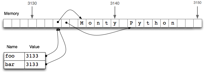
Figure 4.1: List Assignment and Computer Memory: Two list objects foo and bar reference the same location in the computer's memory; updating foo will also modify bar, and vice versa.
The line bar = foo does not copy the contents of the
variable, only its "object reference".
To understand what is going on here, we need to
know how lists are stored in the computer's memory.
In 4.1, we see that a list foo is
a reference to an object stored at location 3133 (which is
itself a series of pointers to other locations holding strings).
When we assign bar = foo, it is just the object reference
3133 that gets copied.
This behavior extends to other aspects of the language, such as
parameter passing (4.4).
Let's experiment some more, by creating a variable empty holding the empty list, then using it three times on the next line.
|
Observe that changing one of the items inside our nested list of lists changed them all. This is because each of the three elements is actually just a reference to one and the same list in memory.
Note
Your Turn: Use multiplication to create a list of lists: nested = [[]] * 3. Now modify one of the elements of the list, and observe that all the elements are changed. Use Python's id() function to find out the numerical identifier for any object, and verify that id(nested[0]), id(nested[1]), and id(nested[2]) are all the same.
Now, notice that when we assign a new value to one of the elements of the list, it does not propagate to the others:
|
We began with a list containing three references to a single empty list object. Then we modified that object by appending 'Python' to it, resulting in a list containing three references to a single list object ['Python']. Next, we overwrote one of those references with a reference to a new object ['Monty']. This last step modified one of the three object references inside the nested list. However, the ['Python'] object wasn't changed, and is still referenced from two places in our nested list of lists. It is crucial to appreciate this difference between modifying an object via an object reference, and overwriting an object reference.
Note
Important: To copy the items from a list foo to a new list bar, you can write bar = foo[:]. This copies the object references inside the list. To copy a structure without copying any object references, use copy.deepcopy().
Equality
Python provides two ways to check that a pair of items are the same. The is operator tests for object identity. We can use it to verify our earlier observations about objects. First we create a list containing several copies of the same object, and demonstrate that they are not only identical according to ==, but also that they are one and the same object:
|
Now let's put a new python in this nest. We can easily show that the objects are not all identical:
|
You can do several pairwise tests to discover which position contains the interloper, but the id() function makes detection easier:
|
This reveals that the second item of the list has a distinct identifier. If you try running this code snippet yourself, expect to see different numbers in the resulting list, and also the interloper may be in a different position.
Having two kinds of equality might seem strange. However, it's really just the type-token distinction, familiar from natural language, here showing up in a programming language.
Conditionals
In the condition part of an if statement, a nonempty string or list is evaluated as true, while an empty string or list evaluates as false.
|
That is, we don't need to say if len(element) > 0: in the condition.
What's the difference between using if...elif as opposed to using a couple of if statements in a row? Well, consider the following situation:
|
Since the if clause of the statement is satisfied, Python never tries to evaluate the elif clause, so we never get to print out 2. By contrast, if we replaced the elif by an if, then we would print out both 1 and 2. So an elif clause potentially gives us more information than a bare if clause; when it evaluates to true, it tells us not only that the condition is satisfied, but also that the condition of the main if clause was not satisfied.
The functions all() and any() can be applied to a list (or other sequence) to check whether all or any items meet some condition:
|
4.2 Sequences
So far, we have seen two kinds of sequence object: strings and lists. Another
kind of sequence is called a tuple.
Tuples are formed with the comma operator , and typically enclosed
using parentheses. We've actually seen them in the
previous chapters, and sometimes referred to them as "pairs", since
there were always two members. However, tuples can have any number
of members. Like lists and strings, tuples can be indexed
and sliced ![[3]](callouts/callout3.gif) , and have a length
, and have a length ![[4]](callouts/callout4.gif) .
.
Caution!
Tuples are constructed using the comma operator. Parentheses are a more general feature of Python syntax, designed for grouping. A tuple containing the single element 'snark' is defined by adding a trailing comma, like this: "'snark',". The empty tuple is a special case, and is defined using empty parentheses ().
Let's compare strings, lists and tuples directly, and do the indexing, slice, and length operation on each type:
|
Notice in this code sample that we computed multiple values on a single line, separated by commas. These comma-separated expressions are actually just tuples — Python allows us to omit the parentheses around tuples if there is no ambiguity. When we print a tuple, the parentheses are always displayed. By using tuples in this way, we are implicitly aggregating items together.
Operating on Sequence Types
We can iterate over the items in a sequence s in a variety of useful ways, as shown in 4.1.
| Python Expression | Comment |
|---|---|
| for item in s | iterate over the items of s |
| for item in sorted(s) | iterate over the items of s in order |
| for item in set(s) | iterate over unique elements of s |
| for item in reversed(s) | iterate over elements of s in reverse |
| for item in set(s).difference(t) | iterate over elements of s not in t |
The sequence functions illustrated in 4.1 can be combined in various ways; for example, to get unique elements of s sorted in reverse, use reversed(sorted(set(s))). We can randomize the contents of a list s before iterating over them, using random.shuffle(s).
We can convert between these sequence types. For example, tuple(s) converts any kind of sequence into a tuple, and list(s) converts any kind of sequence into a list. We can convert a list of strings to a single string using the join() function, e.g. ':'.join(words).
Some other objects, such as a FreqDist, can be converted into a sequence (using list() or sorted()) and support iteration, e.g.
|
In the next example, we use tuples to re-arrange the contents of our list. (We can omit the parentheses because the comma has higher precedence than assignment.)
|
This is an idiomatic and readable way to move items inside a list. It is equivalent to the following traditional way of doing such tasks that does not use tuples (notice that this method needs a temporary variable tmp).
|
As we have seen, Python has sequence functions such as sorted() and reversed() that rearrange the items of a sequence. There are also functions that modify the structure of a sequence and which can be handy for language processing. Thus, zip() takes the items of two or more sequences and "zips" them together into a single list of tuples. Given a sequence s, enumerate(s) returns pairs consisting of an index and the item at that index.
|
Note
It is a widespread feature of Python 3 and NLTK 3 to only perform computation when required (a feature known as "lazy evaluation"). If you ever see a result like <zip object at 0x10d005448> when you expect to see a sequence, you can force the object to be evaluated just by putting it in a context that expects a sequence, like list(x), or for item in x.
For some NLP tasks it is necessary to cut up a sequence into two or more parts.
For instance, we might want to "train" a system on 90% of the data and test it
on the remaining 10%. To do this we decide the location where we want to
cut the data , then cut the sequence at that location .
We can verify that none of the original data is lost during this process, nor is it duplicated
. We can also verify that the ratio of the sizes of the two pieces is what
we intended .
Combining Different Sequence Types
Let's combine our knowledge of these three sequence types, together with list comprehensions, to perform the task of sorting the words in a string by their length.
|
Each of the above lines of code contains a significant feature.
A simple string is actually an object with methods defined on it such as split() .
We use a list comprehension to build a list of tuples ,
where each tuple consists of a number (the word length) and the
word, e.g. (3, 'the'). We use the sort() method
to sort the list in-place. Finally, we discard the length
information and join the words back into a single string .
(The underscore is just a regular Python variable,
but we can use underscore by convention to indicate that we will
not use its value.)
We began by talking about the commonalities in these sequence types, but the above code illustrates important differences in their roles. First, strings appear at the beginning and the end: this is typical in the context where our program is reading in some text and producing output for us to read. Lists and tuples are used in the middle, but for different purposes. A list is typically a sequence of objects all having the same type, of arbitrary length. We often use lists to hold sequences of words. In contrast, a tuple is typically a collection of objects of different types, of fixed length. We often use a tuple to hold a record, a collection of different fields relating to some entity. This distinction between the use of lists and tuples takes some getting used to, so here is another example:
|
Here, a lexicon is represented as a list because it is a collection of objects of a single type — lexical entries — of no predetermined length. An individual entry is represented as a tuple because it is a collection of objects with different interpretations, such as the orthographic form, the part of speech, and the pronunciations (represented in the SAMPA computer-readable phonetic alphabet http://www.phon.ucl.ac.uk/home/sampa/). Note that these pronunciations are stored using a list. (Why?)
Note
A good way to decide when to use tuples vs lists is to ask whether the interpretation of an item depends on its position. For example, a tagged token combines two strings having different interpretation, and we choose to interpret the first item as the token and the second item as the tag. Thus we use tuples like this: ('grail', 'noun'); a tuple of the form ('noun', 'grail') would be nonsensical since it would be a word noun tagged grail. In contrast, the elements of a text are all tokens, and position is not significant. Thus we use lists like this: ['venetian', 'blind']; a list of the form ['blind', 'venetian'] would be equally valid. The linguistic meaning of the words might be different, but the interpretation of list items as tokens is unchanged.
The distinction between lists and tuples has been described in terms of usage. However, there is a more fundamental difference: in Python, lists are mutable, while tuples are immutable. In other words, lists can be modified, while tuples cannot. Here are some of the operations on lists that do in-place modification of the list.
|
Note
Your Turn: Convert lexicon to a tuple, using lexicon = tuple(lexicon), then try each of the above operations, to confirm that none of them is permitted on tuples.
Generator Expressions
We've been making heavy use of list comprehensions, for compact and readable processing of texts. Here's an example where we tokenize and normalize a text:
|
Suppose we now want to process these words further. We can do this by inserting the above
expression inside a call to some other function ,
but Python allows us to omit the brackets .
|
The second line uses a generator expression. This is more than a notational convenience:
in many language processing situations, generator expressions will be more efficient.
In , storage for the list object must be allocated
before the value of max() is computed. If the text is
very large, this could be slow. In , the data is streamed to the calling
function. Since the calling function simply has to find the maximum value — the
word which comes latest in lexicographic sort order — it can process the stream
of data without having to store anything more than the maximum value seen so far.
4.3 Questions of Style
Programming is as much an art as a science. The undisputed "bible" of programming, a 2,500 page multi-volume work by Donald Knuth, is called The Art of Computer Programming. Many books have been written on Literate Programming, recognizing that humans, not just computers, must read and understand programs. Here we pick up on some issues of programming style that have important ramifications for the readability of your code, including code layout, procedural vs declarative style, and the use of loop variables.
Python Coding Style
When writing programs you make many subtle choices about names, spacing, comments, and so on. When you look at code written by other people, needless differences in style make it harder to interpret the code. Therefore, the designers of the Python language have published a style guide for Python code, available at http://www.python.org/dev/peps/pep-0008/. The underlying value presented in the style guide is consistency, for the purpose of maximizing the readability of code. We briefly review some of its key recommendations here, and refer readers to the full guide for detailed discussion with examples.
Code layout should use four spaces per indentation level. You should make sure that when you write Python code in a file, you avoid tabs for indentation, since these can be misinterpreted by different text editors and the indentation can be messed up. Lines should be less than 80 characters long; if necessary you can break a line inside parentheses, brackets, or braces, because Python is able to detect that the line continues over to the next line. If you need to break a line outside parentheses, brackets, or braces, you can often add extra parentheses, and you can always add a backslash at the end of the line that is broken:
|
Note
Typing spaces instead of tabs soon becomes a chore. Many programming editors have built-in support for Python, and can automatically indent code and highlight any syntax errors (including indentation errors). For a list of Python-aware editors, please see http://wiki.python.org/moin/PythonEditors.
Procedural vs Declarative Style
We have just seen how the same task can be performed in different ways, with implications for efficiency. Another factor influencing program development is programming style. Consider the following program to compute the average length of words in the Brown Corpus:
|
In this program we use the variable count to keep track of the number of tokens seen, and total to store the combined length of all words. This is a low-level style, not far removed from machine code, the primitive operations performed by the computer's CPU. The two variables are just like a CPU's registers, accumulating values at many intermediate stages, values that are meaningless until the end. We say that this program is written in a procedural style, dictating the machine operations step by step. Now consider the following program that computes the same thing:
|
The first line uses a generator expression to sum the token lengths, while the second line computes the average as before. Each line of code performs a complete, meaningful task, which can be understood in terms of high-level properties like: "total is the sum of the lengths of the tokens". Implementation details are left to the Python interpreter. The second program uses a built-in function, and constitutes programming at a more abstract level; the resulting code is more declarative. Let's look at an extreme example:
|
The equivalent declarative version uses familiar built-in functions, and its purpose is instantly recognizable:
|
Another case where a loop variable seems to be necessary is for printing a counter with each line of output. Instead, we can use enumerate(), which processes a sequence s and produces a tuple of the form (i, s[i]) for each item in s, starting with (0, s[0]). Here we enumerate the key-value pairs of the frequency distribution, resulting in nested tuples (rank, (word, count)). We print rank+1 so that the counting appears to start from 1, as required when producing a list of ranked items.
|
It's sometimes tempting to use loop variables to store a maximum or minimum value seen so far. Let's use this method to find the longest word in a text.
|
However, a more transparent solution uses two list comprehensions, both having forms that should be familiar by now:
|
Note that our first solution found the first word having the longest length, while the second solution found all of the longest words (which is usually what we would want). Although there's a theoretical efficiency difference between the two solutions, the main overhead is reading the data into main memory; once it's there, a second pass through the data is effectively instantaneous. We also need to balance our concerns about program efficiency with programmer efficiency. A fast but cryptic solution will be harder to understand and maintain.
Some Legitimate Uses for Counters
There are cases where we still want to use loop variables in a list comprehension. For example, we need to use a loop variable to extract successive overlapping n-grams from a list:
|
It is quite tricky to get the range of the loop variable right. Since this is a common operation in NLP, NLTK supports it with functions bigrams(text) and trigrams(text), and a general purpose ngrams(text, n).
Here's an example of how we can use loop variables in building multidimensional structures. For example, to build an array with m rows and n columns, where each cell is a set, we could use a nested list comprehension:
|
Observe that the loop variables i and j are not used anywhere in the resulting object, they are just needed for a syntactically correct for statement. As another example of this usage, observe that the expression ['very' for i in range(3)] produces a list containing three instances of 'very', with no integers in sight.
Note that it would be incorrect to do this work using multiplication, for reasons concerning object copying that were discussed earlier in this section.
|
Iteration is an important programming device. It is tempting to adopt idioms from other languages. However, Python offers some elegant and highly readable alternatives, as we have seen.
4.4 Functions: The Foundation of Structured Programming
Functions provide an effective way to package and re-use program code, as already explained in 3. For example, suppose we find that we often want to read text from an HTML file. This involves several steps: opening the file, reading it in, normalizing whitespace, and stripping HTML markup. We can collect these steps into a function, and give it a name such as get_text(), as shown in 4.2.
| ||
Example 4.2 (code_get_text.py): Figure 4.2: Read text from a file |
Now, any time we want to get cleaned-up text from an HTML file, we can just call get_text() with the name of the file as its only argument. It will return a string, and we can assign this to a variable, e.g.: contents = get_text("test.html"). Each time we want to use this series of steps we only have to call the function.
Using functions has the benefit of saving space in our program. More importantly, our choice of name for the function helps make the program readable. In the case of the above example, whenever our program needs to read cleaned-up text from a file we don't have to clutter the program with four lines of code, we simply need to call get_text(). This naming helps to provide some "semantic interpretation" — it helps a reader of our program to see what the program "means".
Notice that the above function definition contains a string. The first string inside a function definition is called a docstring. Not only does it document the purpose of the function to someone reading the code, it is accessible to a programmer who has loaded the code from a file:
|   >>> help(get_text)
|   Help on function get_text in module __main__:
|
|   get_text(file)
|       Read text from a file, normalizing whitespace and stripping HTML markup.
We have seen that functions help to make our work reusable and readable. They also help make it reliable. When we re-use code that has already been developed and tested, we can be more confident that it handles a variety of cases correctly. We also remove the risk that we forget some important step, or introduce a bug. The program that calls our function also has increased reliability. The author of that program is dealing with a shorter program, and its components behave transparently.
To summarize, as its name suggests, a function captures functionality. It is a segment of code that can be given a meaningful name and which performs a well-defined task. Functions allow us to abstract away from the details, to see a bigger picture, and to program more effectively.
The rest of this section takes a closer look at functions, exploring the mechanics and discussing ways to make your programs easier to read.
Function Inputs and Outputs
We pass information to functions using a function's parameters, the parenthesized list of variables and constants following the function's name in the function definition. Here's a complete example:
|
We first define the function to take two parameters, msg and num
. Then we call the function and pass it two arguments, monty and 3
; these arguments fill the "placeholders" provided by the parameters and
provide values for the occurrences of msg and num in the function body.
It is not necessary to have any parameters, as we see in the following example:
|
A function usually communicates its results back to the calling program via the return statement, as we have just seen. To the calling program, it looks as if the function call had been replaced with the function's result, e.g.:
|
A Python function is not required to have a return statement. Some functions do their work as a side effect, printing a result, modifying a file, or updating the contents of a parameter to the function (such functions are called "procedures" in some other programming languages).
Consider the following three sort functions. The third one is dangerous because a programmer could use it without realizing that it had modified its input. In general, functions should modify the contents of a parameter (my_sort1()), or return a value (my_sort2()), not both (my_sort3()).
|
Parameter Passing
Back in 4.1 you saw that assignment works on values, but that the value of a structured object is a reference to that object. The same is true for functions. Python interprets function parameters as values (this is known as call-by-value). In the following code, set_up() has two parameters, both of which are modified inside the function. We begin by assigning an empty string to w and an empty list to p. After calling the function, w is unchanged, while p is changed:
|
Notice that w was not changed by the function. When we called set_up(w, p), the value of w (an empty string) was assigned to a new variable word. Inside the function, the value of word was modified. However, that change did not propagate to w. This parameter passing is identical to the following sequence of assignments:
|
Let's look at what happened with the list p. When we called set_up(w, p), the value of p (a reference to an empty list) was assigned to a new local variable properties, so both variables now reference the same memory location. The function modifies properties, and this change is also reflected in the value of p as we saw. The function also assigned a new value to properties (the number 5); this did not modify the contents at that memory location, but created a new local variable. This behavior is just as if we had done the following sequence of assignments:
|
Thus, to understand Python's call-by-value parameter passing, it is enough to understand how assignment works. Remember that you can use the id() function and is operator to check your understanding of object identity after each statement.
Variable Scope
Function definitions create a new, local scope for variables. When you assign to a new variable inside the body of a function, the name is only defined within that function. The name is not visible outside the function, or in other functions. This behavior means you can choose variable names without being concerned about collisions with names used in your other function definitions.
When you refer to an existing name from within the body of a function, the Python interpreter first tries to resolve the name with respect to the names that are local to the function. If nothing is found, the interpreter checks if it is a global name within the module. Finally, if that does not succeed, the interpreter checks if the name is a Python built-in. This is the so-called LGB rule of name resolution: local, then global, then built-in.
Caution!
A function can enable access to a global variable using the global declaration. However, this practice should be avoided as much as possible. Defining global variables inside a function introduces dependencies on context and limits the portability (or reusability) of the function. In general you should use parameters for function inputs and return values for function outputs.
Checking Parameter Types
Python does not allow us to declare the type of a variable when we write a program, and this permits us to define functions that are flexible about the type of their arguments. For example, a tagger might expect a sequence of words, but it wouldn't care whether this sequence is expressed as a list or a tuple (or an iterator, another sequence type that is outside the scope of the current discussion).
However, often we want to write programs for later use by others, and want to program in a defensive style, providing useful warnings when functions have not been invoked correctly. The author of the following tag() function assumed that its argument would always be a string.
|
The function returns sensible values for the arguments 'the' and 'knight',
but look what happens when it is passed a list — it fails to
complain, even though the result which it returns is clearly incorrect.
The author of this function could take some extra steps to
ensure that the word parameter of the tag() function is a string.
A naive approach would be to check the type of the argument using
if not type(word) is str, and if word is not a string, to simply
return Python's special empty value, None. This is a slight improvement, because
the function is checking the type of the argument, and trying to return a "special", diagnostic
value for the wrong input.
However, it is also dangerous because the calling program
may not detect that None is intended as a "special" value, and this diagnostic
return value may then be
propagated to other parts of the program with unpredictable consequences.
This approach also fails if the word is a Unicode string, which has
type unicode, not str.
Here's a better solution, using an assert statement together with Python's basestring
type that generalizes over both unicode and str.
|
If the assert statement fails, it will produce an error that cannot be ignored, since it halts program execution. Additionally, the error message is easy to interpret. Adding assertions to a program helps you find logical errors, and is a kind of defensive programming. A more fundamental approach is to document the parameters to each function using docstrings as described later in this section.
Functional Decomposition
Well-structured programs usually make extensive use of functions. When a block of program code grows longer than 10-20 lines, it is a great help to readability if the code is broken up into one or more functions, each one having a clear purpose. This is analogous to the way a good essay is divided into paragraphs, each expressing one main idea.
Functions provide an important kind of abstraction. They allow us to group multiple actions into a single, complex action, and associate a name with it. (Compare this with the way we combine the actions of go and bring back into a single more complex action fetch.) When we use functions, the main program can be written at a higher level of abstraction, making its structure transparent, e.g.
|
Appropriate use of functions makes programs more readable and maintainable. Additionally, it becomes possible to reimplement a function — replacing the function's body with more efficient code — without having to be concerned with the rest of the program.
Consider the freq_words function in 4.3. It updates the contents of a frequency distribution that is passed in as a parameter, and it also prints a list of the n most frequent words.
| ||
| ||
Example 4.3 (code_freq_words1.py): Figure 4.3: Poorly Designed Function to Compute Frequent Words |
This function has a number of problems. The function has two side-effects: it modifies the contents of its second parameter, and it prints a selection of the results it has computed. The function would be easier to understand and to reuse elsewhere if we initialize the FreqDist() object inside the function (in the same place it is populated), and if we moved the selection and display of results to the calling program. Given that its task is to identify frequent words, it should probably just return a list, not the whole frequency distribution. In 4.4 we refactor this function, and simplify its interface by dropping the freqdist parameter.
| ||
| ||
Example 4.4 (code_freq_words2.py): Figure 4.4: Well-Designed Function to Compute Frequent Words |
The readability and usability of the freq_words function is improved.
Note
We have used _ as a variable name. This is no different to any other variable except it signals to the reader that we don't have a use for the information it holds.
Documenting Functions
If we have done a good job at decomposing our program into functions, then it should be easy to describe the purpose of each function in plain language, and provide this in the docstring at the top of the function definition. This statement should not explain how the functionality is implemented; in fact it should be possible to re-implement the function using a different method without changing this statement.
For the simplest functions, a one-line docstring is usually adequate (see 4.2). You should provide a triple-quoted string containing a complete sentence on a single line. For non-trivial functions, you should still provide a one sentence summary on the first line, since many docstring processing tools index this string. This should be followed by a blank line, then a more detailed description of the functionality (see http://www.python.org/dev/peps/pep-0257/ for more information in docstring conventions).
Docstrings can include a doctest block, illustrating the use of the function and the expected output. These can be tested automatically using Python's docutils module. Docstrings should document the type of each parameter to the function, and the return type. At a minimum, that can be done in plain text. However, note that NLTK uses the Sphinx markup language to document parameters. This format can be automatically converted into richly structured API documentation (see http://nltk.org/), and includes special handling of certain "fields" such as param which allow the inputs and outputs of functions to be clearly documented. 4.5 illustrates a complete docstring.
| ||
Example 4.5 (code_sphinx.py): Figure 4.5: Illustration of a complete docstring, consisting of a one-line summary, a more detailed explanation, a doctest example, and Sphinx markup specifying the parameters, types, return type, and exceptions. |
4.5 Doing More with Functions
This section discusses more advanced features, which you may prefer to skip on the first time through this chapter.
Functions as Arguments
So far the arguments we have passed into functions have been simple objects like strings, or structured objects like lists. Python also lets us pass a function as an argument to another function. Now we can abstract out the operation, and apply a different operation on the same data. As the following examples show, we can pass the built-in function len() or a user-defined function last_letter() as arguments to another function:
|
The objects len and last_letter can be passed around like lists and dictionaries. Notice that parentheses are only used after a function name if we are invoking the function; when we are simply treating the function as an object these are omitted.
Python provides us with one more way to define functions as arguments to other functions, so-called lambda expressions. Supposing there was no need to use the above last_letter() function in multiple places, and thus no need to give it a name. We can equivalently write the following:
|
Our next example illustrates passing a function to the sorted() function. When we call the latter with a single argument (the list to be sorted), it uses the built-in comparison function cmp(). However, we can supply our own sort function, e.g. to sort by decreasing length.
|
Accumulative Functions
These functions start by initializing some storage, and iterate over input to build it up, before returning some final object (a large structure or aggregated result). A standard way to do this is to initialize an empty list, accumulate the material, then return the list, as shown in function search1() in 4.6.
| ||
| ||
Example 4.6 (code_search_examples.py): Figure 4.6: Accumulating Output into a List |
The function search2() is a generator. The first time this function is called, it gets as far as the yield statement and pauses. The calling program gets the first word and does any necessary processing. Once the calling program is ready for another word, execution of the function is continued from where it stopped, until the next time it encounters a yield statement. This approach is typically more efficient, as the function only generates the data as it is required by the calling program, and does not need to allocate additional memory to store the output (cf. our discussion of generator expressions above).
Here's a more sophisticated example of a generator which produces
all permutations of a list of words. In order to force the permutations()
function to generate all its output, we wrap it with a call to list() .
|
Higher-Order Functions
Python provides some higher-order functions that are standard features of functional programming languages such as Haskell. We illustrate them here, alongside the equivalent expression using list comprehensions.
Let's start by defining a function is_content_word() which checks whether a word is from the open class of content words. We use this function as the first parameter of filter(), which applies the function to each item in the sequence contained in its second parameter, and only retains the items for which the function returns True.
|
Another higher-order function is map(), which applies a function to every item in a sequence. It is a general version of the extract_property() function we saw in 4.5. Here is a simple way to find the average length of a sentence in the news section of the Brown Corpus, followed by an equivalent version with list comprehension calculation:
|
In the above examples we specified a user-defined function is_content_word() and a built-in function len(). We can also provide a lambda expression. Here's a pair of equivalent examples which count the number of vowels in each word.
|
The solutions based on list comprehensions are usually more readable than the solutions based on higher-order functions, and we have favored the former approach throughout this book.
Named Arguments
When there are a lot of parameters it is easy to get confused about the correct order. Instead we can refer to parameters by name, and even assign them a default value just in case one was not provided by the calling program. Now the parameters can be specified in any order, and can be omitted.
|
These are called keyword arguments. If we mix these two kinds of parameters, then we must ensure that the unnamed parameters precede the named ones. It has to be this way, since unnamed parameters are defined by position. We can define a function that takes an arbitrary number of unnamed and named parameters, and access them via an in-place list of arguments *args and an "in-place dictionary" of keyword arguments **kwargs. (Dictionaries will be presented in 3.)
|
When *args appears as a function parameter, it actually corresponds to all the unnamed parameters of the function. Here's another illustration of this aspect of Python syntax, for the zip() function which operates on a variable number of arguments. We'll use the variable name *song to demonstrate that there's nothing special about the name *args.
|
It should be clear from the above example that typing *song is just a convenient shorthand, and equivalent to typing out song[0], song[1], song[2].
Here's another example of the use of keyword arguments in a function definition, along with three equivalent ways to call the function:
|
A side-effect of having named arguments is that they permit optionality. Thus we can leave out any arguments where we are happy with the default value: freq_words('ch01.rst', min=4), freq_words('ch01.rst', 4). Another common use of optional arguments is to permit a flag. Here's a revised version of the same function that reports its progress if a verbose flag is set:
|
Caution!
Take care not to use a mutable object as the default value of a parameter. A series of calls to the function will use the same object, sometimes with bizarre results as we will see in the discussion of debugging below.
Caution!
If your program will work with a lot of files, it is a good idea to close any open files once they are no longer required. Python will close open files automatically if you use the with statement:
|
4.6 Program Development
Programming is a skill that is acquired over several years of experience with a variety of programming languages and tasks. Key high-level abilities are algorithm design and its manifestation in structured programming. Key low-level abilities include familiarity with the syntactic constructs of the language, and knowledge of a variety of diagnostic methods for trouble-shooting a program which does not exhibit the expected behavior.
This section describes the internal structure of a program module and how to organize a multi-module program. Then it describes various kinds of error that arise during program development, what you can do to fix them and, better still, to avoid them in the first place.
Structure of a Python Module
The purpose of a program module is to bring logically-related definitions and functions together in order to facilitate re-use and abstraction. Python modules are nothing more than individual .py files. For example, if you were working with a particular corpus format, the functions to read and write the format could be kept together. Constants used by both formats, such as field separators, or a EXTN = ".inf" filename extension, could be shared. If the format was updated, you would know that only one file needed to be changed. Similarly, a module could contain code for creating and manipulating a particular data structure such as syntax trees, or code for performing a particular processing task such as plotting corpus statistics.
When you start writing Python modules, it helps to have some examples to emulate. You can locate the code for any NLTK module on your system using the __file__ variable, e.g.:
|
This returns the location of the compiled .pyc file for the module, and you'll probably see a different location on your machine. The file that you will need to open is the corresponding .py source file, and this will be in the same directory as the .pyc file. Alternatively, you can view the latest version of this module on the web at http://code.google.com/p/nltk/source/browse/trunk/nltk/nltk/metrics/distance.py.
Like every other NLTK module, distance.py begins with a group of comment lines giving a one-line title of the module and identifying the authors. (Since the code is distributed, it also includes the URL where the code is available, a copyright statement, and license information.) Next is the module-level docstring, a triple-quoted multiline string containing information about the module that will be printed when someone types help(nltk.metrics.distance).
# Natural Language Toolkit: Distance Metrics
#
# Copyright (C) 2001-2019 NLTK Project
# Author: Edward Loper <edloper@gmail.com>
#         Steven Bird <stevenbird1@gmail.com>
#         Tom Lippincott <tom@cs.columbia.edu>
# URL: <http://nltk.org/>
# For license information, see LICENSE.TXT
#

"""
Distance Metrics.

Compute the distance between two items (usually strings).
As metrics, they must satisfy the following three requirements:

1. d(a, a) = 0
2. d(a, b) >= 0
3. d(a, c) <= d(a, b) + d(b, c)
"""
After this comes all the import statements required for the module, then any global variables, followed by a series of function definitions that make up most of the module. Other modules define "classes," the main building block of object-oriented programming, which falls outside the scope of this book. (Most NLTK modules also include a demo() function which can be used to see examples of the module in use.)
Note
Some module variables and functions are only used within the module. These should have names beginning with an underscore, e.g. _helper(), since this will hide the name. If another module imports this one, using the idiom: from module import *, these names will not be imported. You can optionally list the externally accessible names of a module using a special built-in variable like this: __all__ = ['edit_distance', 'jaccard_distance'].
Multi-Module Programs
Some programs bring together a diverse range of tasks, such as loading data from a corpus, performing some analysis tasks on the data, then visualizing it. We may already have stable modules that take care of loading data and producing visualizations. Our work might involve coding up the analysis task, and just invoking functions from the existing modules. This scenario is depicted in 4.7.
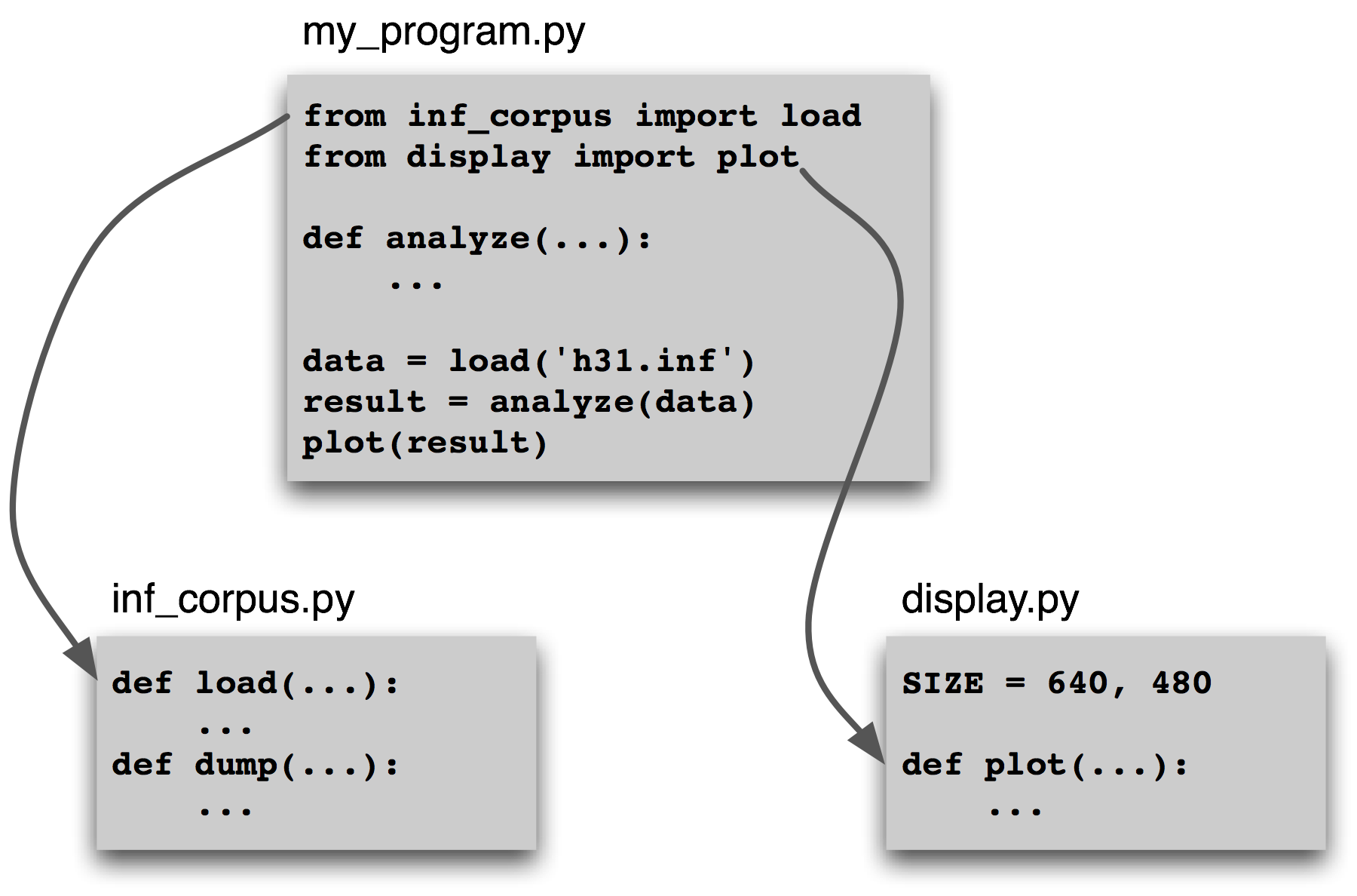
Figure 4.7: Structure of a Multi-Module Program: The main program my_program.py imports functions from two other modules; unique analysis tasks are localized to the main program, while common loading and visualization tasks are kept apart to facilitate re-use and abstraction.
By dividing our work into several modules and using import statements to access functions defined elsewhere, we can keep the individual modules simple and easy to maintain. This approach will also result in a growing collection of modules, and make it possible for us to build sophisticated systems involving a hierarchy of modules. Designing such systems well is a complex software engineering task, and beyond the scope of this book.
Sources of Error
Mastery of programming depends on having a variety of problem-solving skills to draw upon when the program doesn't work as expected. Something as trivial as a mis-placed symbol might cause the program to behave very differently. We call these "bugs" because they are tiny in comparison to the damage they can cause. They creep into our code unnoticed, and it's only much later when we're running the program on some new data that their presence is detected. Sometimes, fixing one bug only reveals another, and we get the distinct impression that the bug is on the move. The only reassurance we have is that bugs are spontaneous and not the fault of the programmer.
Flippancy aside, debugging code is hard because there are so many ways for it to be faulty. Our understanding of the input data, the algorithm, or even the programming language, may be at fault. Let's look at examples of each of these.
First, the input data may contain some unexpected characters. For example, WordNet synset names have the form tree.n.01, with three components separated using periods. The NLTK WordNet module initially decomposed these names using split('.'). However, this method broke when someone tried to look up the word PhD, which has the synset name ph.d..n.01, containing four periods instead of the expected two. The solution was to use rsplit('.', 2) to do at most two splits, using the rightmost instances of the period, and leaving the ph.d. string intact. Although several people had tested the module before it was released, it was some weeks before someone detected the problem (see http://code.google.com/p/nltk/issues/detail?id=297).
Second, a supplied function might not behave as expected. For example, while testing NLTK's interface to WordNet, one of the authors noticed that no synsets had any antonyms defined, even though the underlying database provided a large quantity of antonym information. What looked like a bug in the WordNet interface turned out to be a misunderstanding about WordNet itself: antonyms are defined for lemmas, not for synsets. The only "bug" was a misunderstanding of the interface (see http://code.google.com/p/nltk/issues/detail?id=98).
Third, our understanding of Python's semantics may be at fault. It is easy to make the wrong assumption about the relative scope of two operators. For example, "%s.%s.%02d" % "ph.d.", "n", 1 produces a run-time error TypeError: not enough arguments for format string. This is because the percent operator has higher precedence than the comma operator. The fix is to add parentheses in order to force the required scope. As another example, suppose we are defining a function to collect all tokens of a text having a given length. The function has parameters for the text and the word length, and an extra parameter that allows the initial value of the result to be given as a parameter:
|
The first time we call find_words() , we get all three-letter
words as expected. The second time we specify an initial value for the result,
a one-element list ['ur'], and as expected, the result has this word along with the
other two-letter word in our text. Now, the next time we call find_words()
we use the same parameters as in , but we get a different result!
Each time we call find_words() with no third parameter, the result will
simply extend the result of the previous call, rather than start with the
empty result list as specified in the function definition. The program's
behavior is not as expected because we incorrectly assumed that the default
value was created at the time the function was invoked. However, it is
created just once, at the time the Python interpreter loads the function.
This one list object is used whenever no explicit value is provided to the function.
Debugging Techniques
Since most code errors result from the programmer making incorrect assumptions, the first thing to do when you detect a bug is to check your assumptions. Localize the problem by adding print statements to the program, showing the value of important variables, and showing how far the program has progressed.
If the program produced an "exception" — a run-time error — the interpreter will print a stack trace, pinpointing the location of program execution at the time of the error. If the program depends on input data, try to reduce this to the smallest size while still producing the error.
Once you have localized the problem to a particular function, or to a line of code, you need to work out what is going wrong. It is often helpful to recreate the situation using the interactive command line. Define some variables then copy-paste the offending line of code into the session and see what happens. Check your understanding of the code by reading some documentation, and examining other code samples that purport to do the same thing that you are trying to do. Try explaining your code to someone else, in case they can see where things are going wrong.
Python provides a debugger which allows you to monitor the execution of your program, specify line numbers where execution will stop (i.e. breakpoints), and step through sections of code and inspect the value of variables. You can invoke the debugger on your code as follows:
|
It will present you with a prompt (Pdb) where you can type instructions to the debugger. Type help to see the full list of commands. Typing step (or just s) will execute the current line and stop. If the current line calls a function, it will enter the function and stop at the first line. Typing next (or just n) is similar, but it stops execution at the next line in the current function. The break (or b) command can be used to create or list breakpoints. Type continue (or c) to continue execution as far as the next breakpoint. Type the name of any variable to inspect its value.
We can use the Python debugger to locate the problem in our find_words()
function. Remember that the problem arose the second time the function was
called. We'll start by calling the function without using the debugger ,
using the smallest possible input. The second time, we'll call it with the
debugger .
|
Here we typed just two commands into the debugger: step took us inside the function, and args showed the values of its arguments (or parameters). We see immediately that result has an initial value of ['cat'], and not the empty list as expected. The debugger has helped us to localize the problem, prompting us to check our understanding of Python functions.
Defensive Programming
In order to avoid some of the pain of debugging, it helps to adopt some defensive programming habits. Instead of writing a 20-line program then testing it, build the program bottom-up out of small pieces that are known to work. Each time you combine these pieces to make a larger unit, test it carefully to see that it works as expected. Consider adding assert statements to your code, specifying properties of a variable, e.g. assert(isinstance(text, list)). If the value of the text variable later becomes a string when your code is used in some larger context, this will raise an AssertionError and you will get immediate notification of the problem.
Once you think you've found the bug, view your solution as a hypothesis. Try to predict the effect of your bugfix before re-running the program. If the bug isn't fixed, don't fall into the trap of blindly changing the code in the hope that it will magically start working again. Instead, for each change, try to articulate a hypothesis about what is wrong and why the change will fix the problem. Then undo the change if the problem was not resolved.
As you develop your program, extend its functionality, and fix any bugs, it helps to maintain a suite of test cases. This is called regression testing, since it is meant to detect situations where the code "regresses" — where a change to the code has an unintended side-effect of breaking something that used to work. Python provides a simple regression testing framework in the form of the doctest module. This module searches a file of code or documentation for blocks of text that look like an interactive Python session, of the form you have already seen many times in this book. It executes the Python commands it finds, and tests that their output matches the output supplied in the original file. Whenever there is a mismatch, it reports the expected and actual values. For details please consult the doctest documentation at http://docs.python.org/library/doctest.html. Apart from its value for regression testing, the doctest module is useful for ensuring that your software documentation stays in sync with your code.
Perhaps the most important defensive programming strategy is to set out your code clearly, choose meaningful variable and function names, and simplify the code wherever possible by decomposing it into functions and modules with well-documented interfaces.
4.7 Algorithm Design
This section discusses more advanced concepts, which you may prefer to skip on the first time through this chapter.
A major part of algorithmic problem solving is selecting or adapting an appropriate algorithm for the problem at hand. Sometimes there are several alternatives, and choosing the best one depends on knowledge about how each alternative performs as the size of the data grows. Whole books are written on this topic, and we only have space to introduce some key concepts and elaborate on the approaches that are most prevalent in natural language processing.
The best known strategy is known as divide-and-conquer. We attack a problem of size n by dividing it into two problems of size n/2, solve these problems, and combine their results into a solution of the original problem. For example, suppose that we had a pile of cards with a single word written on each card. We could sort this pile by splitting it in half and giving it to two other people to sort (they could do the same in turn). Then, when two sorted piles come back, it is an easy task to merge them into a single sorted pile. See 4.8 for an illustration of this process.
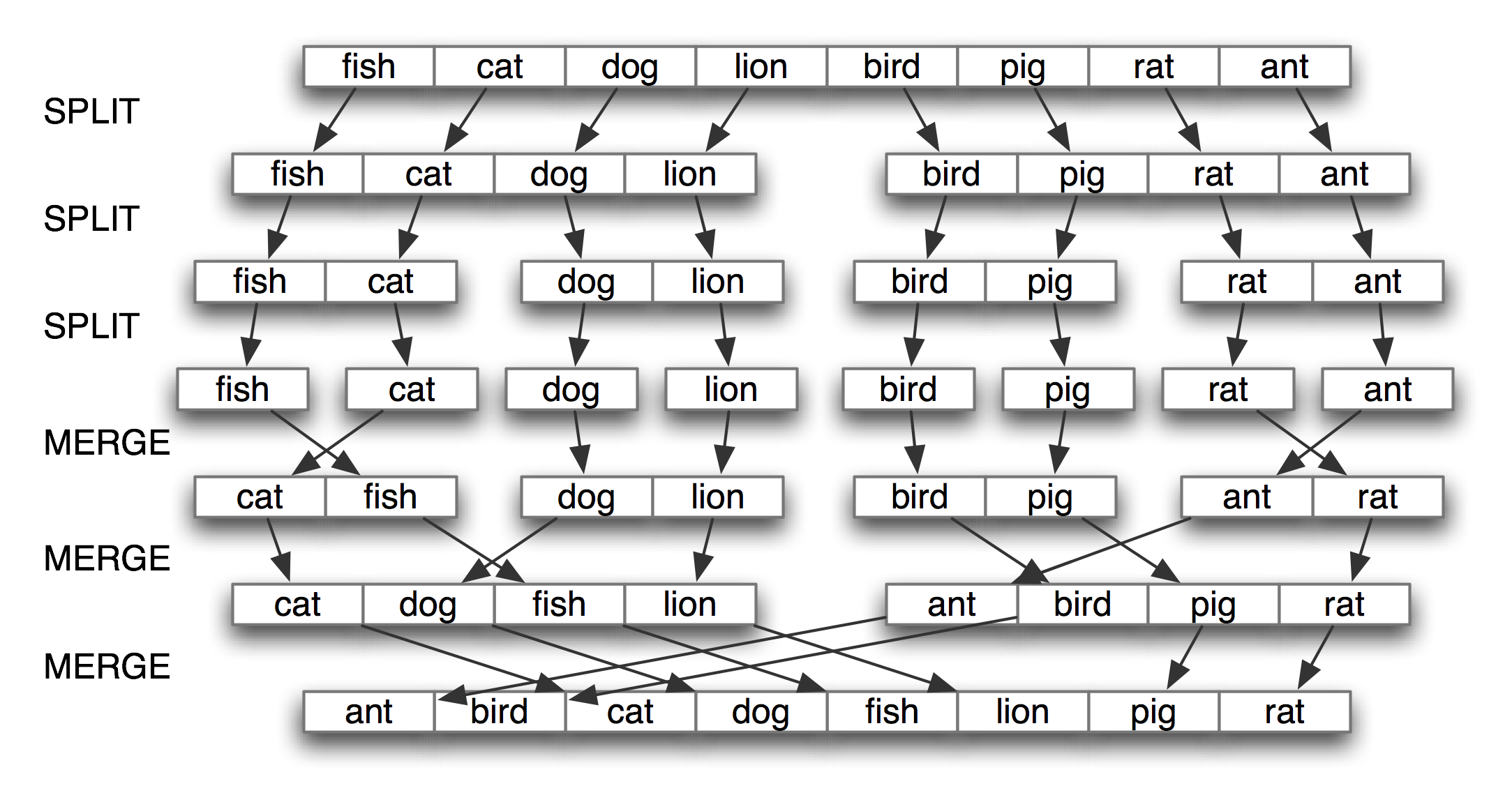
Figure 4.8: Sorting by Divide-and-Conquer: to sort an array, we split it in half and sort each half (recursively); we merge each sorted half back into a whole list (again recursively); this algorithm is known as "Merge Sort".
Another example is the process of looking up a word in a dictionary. We open the book somewhere around the middle and compare our word with the current page. If it's earlier in the dictionary we repeat the process on the first half; if its later we use the second half. This search method is called binary search since it splits the problem in half at every step.
In another approach to algorithm design, we attack a problem by transforming it into an instance of a problem we already know how to solve. For example, in order to detect duplicate entries in a list, we can pre-sort the list, then scan through it once to check if any adjacent pairs of elements are identical.
Recursion
The above examples of sorting and searching have a striking property: to solve a problem of size n, we have to break it in half and then work on one or more problems of size n/2. A common way to implement such methods uses recursion. We define a function f which simplifies the problem, and calls itself to solve one or more easier instances of the same problem. It then combines the results into a solution for the original problem.
For example, suppose we have a set of n words, and want to calculate how many different ways they can be combined to make a sequence of words. If we have only one word (n=1), there is just one way to make it into a sequence. If we have a set of two words, there are two ways to put them into a sequence. For three words there are six possibilities. In general, for n words, there are n × n-1 × … × 2 × 1 ways (i.e. the factorial of n). We can code this up as follows:
|
However, there is also a recursive algorithm for solving this problem, based on the following observation. Suppose we have a way to construct all orderings for n-1 distinct words. Then for each such ordering, there are n places where we can insert a new word: at the start, the end, or any of the n-2 boundaries between the words. Thus we simply multiply the number of solutions found for n-1 by the value of n. We also need the base case, to say that if we have a single word, there's just one ordering. We can code this up as follows:
|
These two algorithms solve the same problem. One uses iteration while the other uses recursion. We can use recursion to navigate a deeply-nested object, such as the WordNet hypernym hierarchy. Let's count the size of the hypernym hierarchy rooted at a given synset s. We'll do this by finding the size of each hyponym of s, then adding these together (we will also add 1 for the synset itself). The following function size1() does this work; notice that the body of the function includes a recursive call to size1():
|
We can also design an iterative solution to this problem which processes
the hierarchy in layers. The first layer is the synset itself ,
then all the hyponyms of the synset, then all the hyponyms of the
hyponyms. Each time through the loop it computes the next layer
by finding the hyponyms of everything in the last layer .
It also maintains a total of the number of synsets encountered so far .
|
Not only is the iterative solution much longer, it is harder to interpret. It forces us to think procedurally, and keep track of what is happening with the layer and total variables through time. Let's satisfy ourselves that both solutions give the same result. We'll use another form of the import statement, allowing us to abbreviate the name wordnet to wn:
|
As a final example of recursion, let's use it to construct a deeply-nested object. A letter trie is a data structure that can be used for indexing a lexicon, one letter at a time. (The name is based on the word retrieval). For example, if trie contained a letter trie, then trie['c'] would be a smaller trie which held all words starting with c. 4.9 demonstrates the recursive process of building a trie, using Python dictionaries (3). To insert the word chien (French for dog), we split off the c and recursively insert hien into the sub-trie trie['c']. The recursion continues until there are no letters remaining in the word, when we store the intended value (in this case, the word dog).
| ||
| ||
Example 4.9 (code_trie.py): Figure 4.9: Building a Letter Trie: A recursive function that builds a nested dictionary structure; each level of nesting contains all words with a given prefix, and a sub-trie containing all possible continuations. |
Caution!
Despite the simplicity of recursive programming, it comes with a cost. Each time a function is called, some state information needs to be pushed on a stack, so that once the function has completed, execution can continue from where it left off. For this reason, iterative solutions are often more efficient than recursive solutions.
Space-Time Tradeoffs
We can sometimes significantly speed up the execution of a program by building an auxiliary data structure, such as an index. The listing in 4.10 implements a simple text retrieval system for the Movie Reviews Corpus. By indexing the document collection it provides much faster lookup.
| ||
Example 4.10 (code_search_documents.py): Figure 4.10: A Simple Text Retrieval System |
A more subtle example of a space-time tradeoff involves replacing the tokens of a corpus with integer identifiers. We create a vocabulary for the corpus, a list in which each word is stored once, then invert this list so that we can look up any word to find its identifier. Each document is preprocessed, so that a list of words becomes a list of integers. Any language models can now work with integers. See the listing in 4.11 for an example of how to do this for a tagged corpus.
| ||
Example 4.11 (code_strings_to_ints.py): Figure 4.11: Preprocess tagged corpus data, converting all words and tags to integers |
Another example of a space-time tradeoff is maintaining a vocabulary list. If you need to process an input text to check that all words are in an existing vocabulary, the vocabulary should be stored as a set, not a list. The elements of a set are automatically indexed, so testing membership of a large set will be much faster than testing membership of the corresponding list.
We can test this claim using the timeit module.
The Timer class has two parameters, a statement which
is executed multiple times, and setup code that is executed
once at the beginning. We will simulate a vocabulary of
100,000 items using a list or set
of integers. The test statement will generate a random
item which has a 50% chance of being in the vocabulary .
|
Performing 1000 list membership tests takes a total of 2.8 seconds, while the equivalent tests on a set take a mere 0.0037 seconds, or three orders of magnitude faster!
Dynamic Programming
Dynamic programming is a general technique for designing algorithms which is widely used in natural language processing. The term 'programming' is used in a different sense to what you might expect, to mean planning or scheduling. Dynamic programming is used when a problem contains overlapping sub-problems. Instead of computing solutions to these sub-problems repeatedly, we simply store them in a lookup table. In the remainder of this section we will introduce dynamic programming, but in a rather different context to syntactic parsing.
Pingala was an Indian author who lived around the 5th century B.C., and wrote a treatise on Sanskrit prosody called the Chandas Shastra. Virahanka extended this work around the 6th century A.D., studying the number of ways of combining short and long syllables to create a meter of length n. Short syllables, marked S, take up one unit of length, while long syllables, marked L, take two. Pingala found, for example, that there are five ways to construct a meter of length 4: V4 = {LL, SSL, SLS, LSS, SSSS}. Observe that we can split V4 into two subsets, those starting with L and those starting with S, as shown in (1).
| (1) | V4 = LL, LSS i.e. L prefixed to each item of V2 = {L, SS} SSL, SLS, SSSS i.e. S prefixed to each item of V3 = {SL, LS, SSS} |
| ||
| ||
Example 4.12 (code_virahanka.py): Figure 4.12: Four Ways to Compute Sanskrit Meter: (i) recursive; (ii) bottom-up dynamic programming; (iii) top-down dynamic programming; and (iv) built-in memoization. |
With this observation, we can write a little recursive function called virahanka1() to compute these meters, shown in 4.12. Notice that, in order to compute V4 we first compute V3 and V2. But to compute V3, we need to first compute V2 and V1. This call structure is depicted in (2).
| (2) | 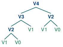 |
As you can see, V2 is computed twice. This might not seem like a significant problem, but it turns out to be rather wasteful as n gets large: to compute V20 using this recursive technique, we would compute V2 4,181 times; and for V40 we would compute V2 63,245,986 times! A much better alternative is to store the value of V2 in a table and look it up whenever we need it. The same goes for other values, such as V3 and so on. Function virahanka2() implements a dynamic programming approach to the problem. It works by filling up a table (called lookup) with solutions to all smaller instances of the problem, stopping as soon as we reach the value we're interested in. At this point we read off the value and return it. Crucially, each sub-problem is only ever solved once.
Notice that the approach taken in virahanka2() is to solve smaller problems on the way to solving larger problems. Accordingly, this is known as the bottom-up approach to dynamic programming. Unfortunately it turns out to be quite wasteful for some applications, since it may compute solutions to sub-problems that are never required for solving the main problem. This wasted computation can be avoided using the top-down approach to dynamic programming, which is illustrated in the function virahanka3() in 4.12. Unlike the bottom-up approach, this approach is recursive. It avoids the huge wastage of virahanka1() by checking whether it has previously stored the result. If not, it computes the result recursively and stores it in the table. The last step is to return the stored result. The final method, in virahanka4(), is to use a Python "decorator" called memoize, which takes care of the housekeeping work done by virahanka3() without cluttering up the program. This "memoization" process stores the result of each previous call to the function along with the parameters that were used. If the function is subsequently called with the same parameters, it returns the stored result instead of recalculating it. (This aspect of Python syntax is beyond the scope of this book.)
This concludes our brief introduction to dynamic programming. We will encounter it again in 4.
4.8 A Sample of Python Libraries
Python has hundreds of third-party libraries, specialized software packages that extend the functionality of Python. NLTK is one such library. To realize the full power of Python programming, you should become familiar with several other libraries. Most of these will need to be manually installed on your computer.
Matplotlib
Python has some libraries that are useful for visualizing language data. The Matplotlib package supports sophisticated plotting functions with a MATLAB-style interface, and is available from http://matplotlib.sourceforge.net/.
So far we have focused on textual presentation and the use of formatted print statements to get output lined up in columns. It is often very useful to display numerical data in graphical form, since this often makes it easier to detect patterns. For example, in 3.7 we saw a table of numbers showing the frequency of particular modal verbs in the Brown Corpus, classified by genre. The program in 4.13 presents the same information in graphical format. The output is shown in 4.14 (a color figure in the graphical display).
| ||
| ||
Example 4.13 (code_modal_plot.py): Figure 4.13: Frequency of Modals in Different Sections of the Brown Corpus |
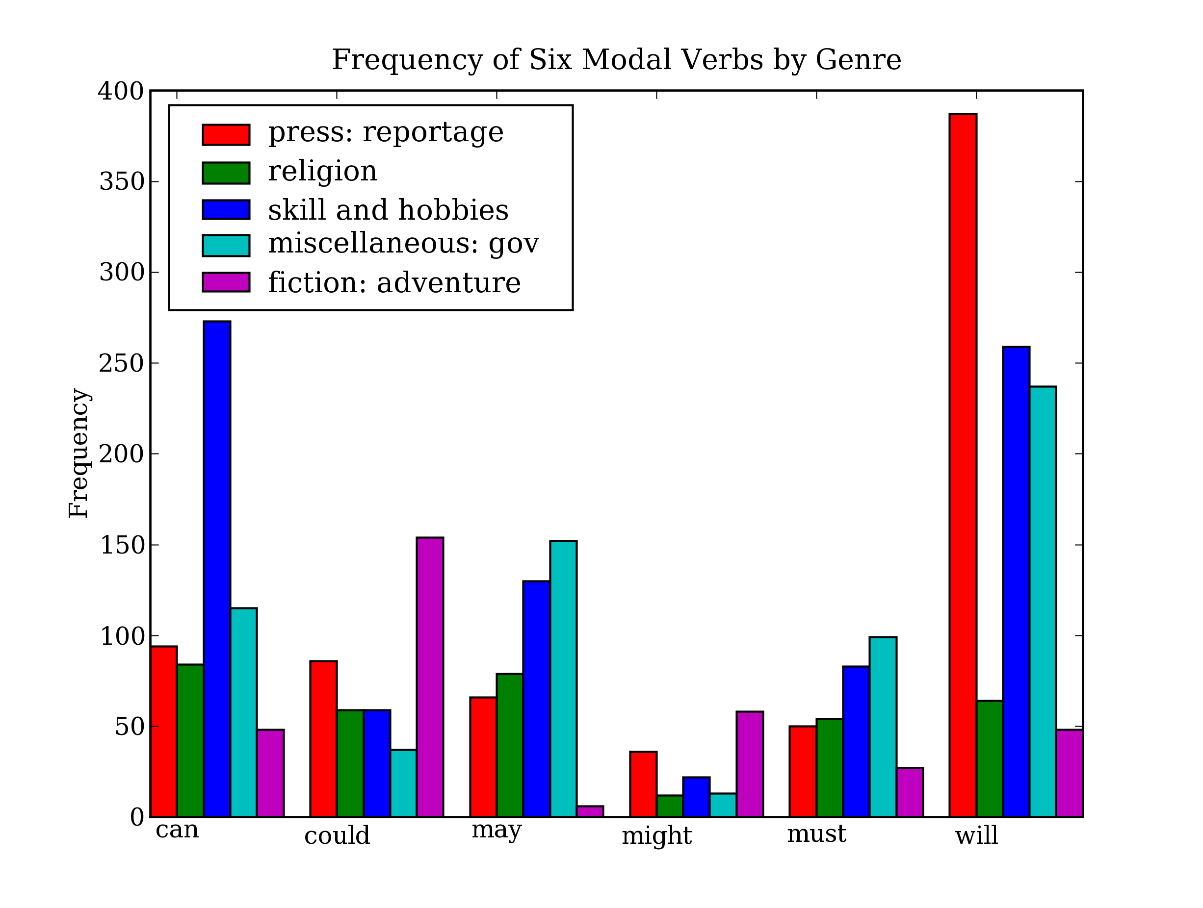
Figure 4.14: Bar Chart Showing Frequency of Modals in Different Sections of Brown Corpus: this visualization was produced by the program in 4.13.
From the bar chart it is immediately obvious that may and must have almost identical relative frequencies. The same goes for could and might.
It is also possible to generate such data visualizations on the fly.
For example, a web page with form input could permit visitors to specify
search parameters, submit the form, and see a dynamically generated
visualization.
To do this we have to specify the Agg backend for matplotlib,
which is a library for producing raster (pixel) images .
Next, we use all the same Matplotlib methods as before, but instead of displaying the
result on a graphical terminal using pyplot.show(), we save it to a file
using pyplot.savefig() . We specify the filename
then print HTML markup that directs the web browser to load the file.
NetworkX
The NetworkX package is for defining and manipulating structures consisting of
nodes and edges, known as graphs. It is
available from https://networkx.lanl.gov/.
NetworkX can be used in conjunction with Matplotlib to
visualize networks, such as WordNet (the semantic network we
introduced in 5). The program in 4.15
initializes an empty graph then traverses
the WordNet hypernym hierarchy adding edges to
the graph .
Notice that the traversal is recursive ,
applying the programming technique discussed in
4.7. The resulting display is shown in 4.16.
| ||
| ||
Example 4.15 (code_networkx.py): Figure 4.15: Using the NetworkX and Matplotlib Libraries |
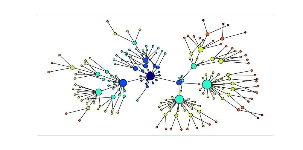
Figure 4.16: Visualization with NetworkX and Matplotlib: Part of the WordNet hypernym hierarchy is displayed, starting with dog.n.01 (the darkest node in the middle); node size is based on the number of children of the node, and color is based on the distance of the node from dog.n.01; this visualization was produced by the program in 4.15.
csv
Language analysis work often involves data tabulations, containing information about lexical items, or the participants in an empirical study, or the linguistic features extracted from a corpus. Here's a fragment of a simple lexicon, in CSV format:
We can use Python's CSV library to read and write files stored in this format.
For example, we can open a CSV file called lexicon.csv
and iterate over its rows :
|
Each row is just a list of strings. If any fields contain numerical data, they will appear as strings, and will have to be converted using int() or float().
NumPy
The NumPy package provides substantial support for numerical processing in Python. NumPy has a multi-dimensional array object, which is easy to initialize and access:
|
NumPy includes linear algebra functions. Here we perform singular value decomposition on a matrix, an operation used in latent semantic analysis to help identify implicit concepts in a document collection.
|
NLTK's clustering package nltk.cluster makes extensive use of NumPy arrays, and includes support for k-means clustering, Gaussian EM clustering, group average agglomerative clustering, and dendrogram plots. For details, type help(nltk.cluster).
Other Python Libraries
There are many other Python libraries, and you can search for them with the help of the Python Package Index http://pypi.python.org/. Many libraries provide an interface to external software, such as relational databases (e.g. mysql-python) and large document collections (e.g. PyLucene). Many other libraries give access to file formats such as PDF, MSWord, and XML (pypdf, pywin32, xml.etree), RSS feeds (e.g. feedparser), and electronic mail (e.g. imaplib, email).
4.9 Summary
- Python's assignment and parameter passing use object references; e.g. if a is a list and we assign b = a, then any operation on a will modify b, and vice versa.
- The is operation tests if two objects are identical internal objects, while == tests if two objects are equivalent. This distinction parallels the type-token distinction.
- Strings, lists and tuples are different kinds of sequence object, supporting common operations such as indexing, slicing, len(), sorted(), and membership testing using in.
- A declarative programming style usually produces more compact, readable code; manually-incremented loop variables are usually unnecessary; when a sequence must be enumerated, use enumerate().
- Functions are an essential programming abstraction: key concepts to understand are parameter passing, variable scope, and docstrings.
- A function serves as a namespace: names defined inside a function are not visible outside that function, unless those names are declared to be global.
- Modules permit logically-related material to be localized in a file. A module serves as a namespace: names defined in a module — such as variables and functions — are not visible to other modules, unless those names are imported.
- Dynamic programming is an algorithm design technique used widely in NLP that stores the results of previous computations in order to avoid unnecessary recomputation.
4.10 Further Reading
This chapter has touched on many topics in programming, some specific to Python, and some quite general. We've just scratched the surface, and you may want to read more about these topics, starting with the further materials for this chapter available at http://nltk.org/.
The Python website provides extensive documentation. It is important to understand the built-in functions and standard types, described at http://docs.python.org/library/functions.html and http://docs.python.org/library/stdtypes.html. We have learnt about generators and their importance for efficiency; for information about iterators, a closely related topic, see http://docs.python.org/library/itertools.html. Consult your favorite Python book for more information on such topics. An excellent resource for using Python for multimedia processing, including working with sound files, is (Guzdial, 2005).
When using the online Python documentation, be aware that your installed version might be different from the version of the documentation you are reading. You can easily check what version you have, with import sys; sys.version. Version-specific documentation is available at http://www.python.org/doc/versions/.
Algorithm design is a rich field within computer science. Some good starting points are (Harel, 2004), (Levitin, 2004), (Knuth, 2006). Useful guidance on the practice of software development is provided in (Hunt & Thomas, 2000) and (McConnell, 2004).
4.11 Exercises
☼ Find out more about sequence objects using Python's help facility. In the interpreter, type help(str), help(list), and help(tuple). This will give you a full list of the functions supported by each type. Some functions have special names flanked with underscore; as the help documentation shows, each such function corresponds to something more familiar. For example x.__getitem__(y) is just a long-winded way of saying x[y].
☼ Identify three operations that can be performed on both tuples and lists. Identify three list operations that cannot be performed on tuples. Name a context where using a list instead of a tuple generates a Python error.
☼ Find out how to create a tuple consisting of a single item. There are at least two ways to do this.
☼ Create a list words = ['is', 'NLP', 'fun', '?']. Use a series of assignment statements (e.g. words[1] = words[2]) and a temporary variable tmp to transform this list into the list ['NLP', 'is', 'fun', '!']. Now do the same transformation using tuple assignment.
☼ Read about the built-in comparison function cmp, by typing help(cmp). How does it differ in behavior from the comparison operators?
☼ Does the method for creating a sliding window of n-grams behave correctly for the two limiting cases: n = 1, and n = len(sent)?
☼ We pointed out that when empty strings and empty lists occur in the condition part of an if clause, they evaluate to False. In this case, they are said to be occurring in a Boolean context. Experiment with different kind of non-Boolean expressions in Boolean contexts, and see whether they evaluate as True or False.
☼ Use the inequality operators to compare strings, e.g. 'Monty' < 'Python'. What happens when you do 'Z' < 'a'? Try pairs of strings which have a common prefix, e.g. 'Monty' < 'Montague'. Read up on "lexicographical sort" in order to understand what is going on here. Try comparing structured objects, e.g. ('Monty', 1) < ('Monty', 2). Does this behave as expected?
☼ Write code that removes whitespace at the beginning and end of a string, and normalizes whitespace between words to be a single space character.
- do this task using split() and join()
- do this task using regular expression substitutions
☼ Write a program to sort words by length. Define a helper function cmp_len which uses the cmp comparison function on word lengths.
◑ Create a list of words and store it in a variable sent1. Now assign sent2 = sent1. Modify one of the items in sent1 and verify that sent2 has changed.
- Now try the same exercise but instead assign sent2 = sent1[:]. Modify sent1 again and see what happens to sent2. Explain.
- Now define text1 to be a list of lists of strings (e.g. to represent a text consisting of multiple sentences. Now assign text2 = text1[:], assign a new value to one of the words, e.g. text1[1][1] = 'Monty'. Check what this did to text2. Explain.
- Load Python's deepcopy() function (i.e. from copy import deepcopy), consult its documentation, and test that it makes a fresh copy of any object.
◑ Initialize an n-by-m list of lists of empty strings using list multiplication, e.g. word_table = [[''] * n] * m. What happens when you set one of its values, e.g. word_table[1][2] = "hello"? Explain why this happens. Now write an expression using range() to construct a list of lists, and show that it does not have this problem.
◑ Write code to initialize a two-dimensional array of sets called word_vowels and process a list of words, adding each word to word_vowels[l][v] where l is the length of the word and v is the number of vowels it contains.
◑ Write a function novel10(text) that prints any word that appeared in the last 10% of a text that had not been encountered earlier.
◑ Write a program that takes a sentence expressed as a single string, splits it and counts up the words. Get it to print out each word and the word's frequency, one per line, in alphabetical order.
◑ Read up on Gematria, a method for assigning numbers to words, and for mapping between words having the same number to discover the hidden meaning of texts (http://en.wikipedia.org/wiki/Gematria, http://essenes.net/gemcal.htm).
Write a function gematria() that sums the numerical values of the letters of a word, according to the letter values in letter_vals:
>>> letter_vals = {'a':1, 'b':2, 'c':3, 'd':4, 'e':5, 'f':80, 'g':3, 'h':8,
... 'i':10, 'j':10, 'k':20, 'l':30, 'm':40, 'n':50, 'o':70, 'p':80, 'q':100,
... 'r':200, 's':300, 't':400, 'u':6, 'v':6, 'w':800, 'x':60, 'y':10, 'z':7}
Process a corpus (e.g. nltk.corpus.state_union) and for each document, count how many of its words have the number 666.
Write a function decode() to process a text, randomly replacing words with their Gematria equivalents, in order to discover the "hidden meaning" of the text.
◑ Write a function shorten(text, n) to process a text, omitting the n most frequently occurring words of the text. How readable is it?
◑ Write code to print out an index for a lexicon, allowing someone to look up words according to their meanings (or pronunciations; whatever properties are contained in lexical entries).
◑ Write a list comprehension that sorts a list of WordNet synsets for proximity to a given synset. For example, given the synsets minke_whale.n.01, orca.n.01, novel.n.01, and tortoise.n.01, sort them according to their shortest_path_distance() from right_whale.n.01.
◑ Write a function that takes a list of words (containing duplicates) and returns a list of words (with no duplicates) sorted by decreasing frequency. E.g. if the input list contained 10 instances of the word table and 9 instances of the word chair, then table would appear before chair in the output list.
◑ Write a function that takes a text and a vocabulary as its arguments and returns the set of words that appear in the text but not in the vocabulary. Both arguments can be represented as lists of strings. Can you do this in a single line, using set.difference()?
◑ Import the itemgetter() function from the operator module in Python's standard library (i.e. from operator import itemgetter). Create a list words containing several words. Now try calling: sorted(words, key=itemgetter(1)), and sorted(words, key=itemgetter(-1)). Explain what itemgetter() is doing.
◑ Write a recursive function lookup(trie, key) that looks up a key in a trie, and returns the value it finds. Extend the function to return a word when it is uniquely determined by its prefix (e.g. vanguard is the only word that starts with vang-, so lookup(trie, 'vang') should return the same thing as lookup(trie, 'vanguard')).
◑ Read up on "keyword linkage" (chapter 5 of (Scott & Tribble, 2006)). Extract keywords from NLTK's Shakespeare Corpus and using the NetworkX package, plot keyword linkage networks.
◑ Read about string edit distance and the Levenshtein Algorithm. Try the implementation provided in nltk.edit_distance(). In what way is this using dynamic programming? Does it use the bottom-up or top-down approach? [See also http://norvig.com/spell-correct.html]
◑ The Catalan numbers arise in many applications of combinatorial mathematics, including the counting of parse trees (6). The series can be defined as follows: C0 = 1, and Cn+1 = Σ0..n (CiCn-i).
- Write a recursive function to compute nth Catalan number Cn.
- Now write another function that does this computation using dynamic programming.
- Use the timeit module to compare the performance of these functions as n increases.
★ Reproduce some of the results of (Zhao & Zobel, 2007) concerning authorship identification.
★ Study gender-specific lexical choice, and see if you can reproduce some of the results of http://www.clintoneast.com/articles/words.php
★ Write a recursive function that pretty prints a trie in alphabetically sorted order, e.g.:
chair: 'flesh'
---t: 'cat'
--ic: 'stylish'
---en: 'dog'
★ With the help of the trie data structure, write a recursive function that processes text, locating the uniqueness point in each word, and discarding the remainder of each word. How much compression does this give? How readable is the resulting text?
★ Obtain some raw text, in the form of a single, long string. Use Python's textwrap module to break it up into multiple lines. Now write code to add extra spaces between words, in order to justify the output. Each line must have the same width, and spaces must be approximately evenly distributed across each line. No line can begin or end with a space.
★ Develop a simple extractive summarization tool, that prints the sentences of a document which contain the highest total word frequency. Use FreqDist() to count word frequencies, and use sum to sum the frequencies of the words in each sentence. Rank the sentences according to their score. Finally, print the n highest-scoring sentences in document order. Carefully review the design of your program, especially your approach to this double sorting. Make sure the program is written as clearly as possible.
★ Read the following article on semantic orientation of adjectives. Use the NetworkX package to visualize a network of adjectives with edges to indicate same vs different semantic orientation. http://www.aclweb.org/anthology/P97-1023
★ Design an algorithm to find the "statistically improbable phrases" of a document collection. http://www.amazon.com/gp/search-inside/sipshelp.html
★ Write a program to implement a brute-force algorithm for discovering word squares, a kind of n × n crossword in which the entry in the nth row is the same as the entry in the nth column. For discussion, see http://itre.cis.upenn.edu/~myl/languagelog/archives/002679.html
About this document...
UPDATED FOR NLTK 3.0. This is a chapter from Natural Language Processing with Python, by Steven Bird, Ewan Klein and Edward Loper, Copyright © 2019 the authors. It is distributed with the Natural Language Toolkit [http://nltk.org/], Version 3.0, under the terms of the Creative Commons Attribution-Noncommercial-No Derivative Works 3.0 United States License [http://creativecommons.org/licenses/by-nc-nd/3.0/us/].
This document was built on Wed 4 Sep 2019 11:40:48 ACST